Oscillations - Part 2
Damping
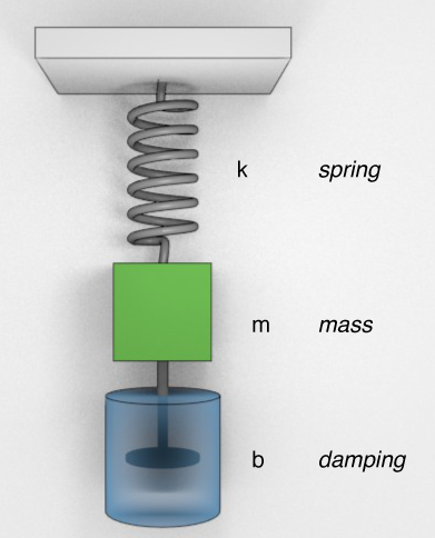
Spring-Mass-Damper system
Let's add more terms!
$$F = m \ddot{x} = -kx - b \dot{x}$$Clean it up:
\begin{equation} \ddot{x} + 2 \beta \dot{x} + w_0^2 x = 0 \label{eq:dampedoscillatoreqofmotion} \end{equation} where $\beta \equiv \frac{b}{2m}$ and $\omega_0 \equiv \sqrt{\frac{k}{m}}$
Note: $\omega_0$ is the natural frequency.
This is a second-order, linear, differential equation. It's solvable if we stipulate two initial conditions: $$x(0) = x_0$$ and $$v(0) = v_0$$
A general solution would look like: $$x \propto e^{\alpha t}$$
If we put this in for $x$, we would get: $$\frac{d^2}{dt^2}(e^{\alpha t}) + 2 \beta \frac{d}{dt}(e^{\alpha t}) + \omega_0^2 e^{\alpha t} = 0 $$ which would become, after taking the first and second derivatives of the exponentials: \begin{equation} \alpha^2 + 2 \beta \alpha + \omega_0^2 = 0 \end{equation} This is just a quadratic equation in $\alpha$ so we can write the solution to $\alpha$
Thus, a general solution would consist of the two independent solutions: \begin{equation} x(t) = C_1 e^{\left( -\beta + \sqrt{\beta^2 - \omega_0^2 }\right) t} + C_2 e^{\left(-\beta - \sqrt{\beta^2 - \omega_0^2}\right) t} \end{equation} or
There are 3 possibilities now:
- Overdamped: $\beta \gt \omega_0$
- Critically Damped: $\beta = \omega_0$
- Underdamped: $\beta \lt \omega_0$
(plus the $\beta = 0$ case.)
Overdamped
If $$\beta \gt \omega_0$$ then the exponent $\alpha$ in our solution $x = e^{\alpha t}$ will be negative and real.
This means we can write our general solution as the sum of two terms: $$x(t) = C_1 e^{\gamma_1 t}+ C_2 e^{\gamma_2 t}$$ Where $$ \begin{align} \gamma_1 & = -\beta + \sqrt{\beta^2 - \omega_0^2} \\ \gamma_2 & = -\beta - \sqrt{\beta^2 - \omega_0^2} \end{align} $$ The constants $C_1$ and $C_2$ will be determined by the initial conditions of the oscillator, i.e. $x(t = 0)$ and $\dot{x}(t = 0)$.

Overdamped oscillator
What if $x_0 = 0$ and $v_{0x} \neq 0$?

Dependence on $\beta$.
Here we are plotting the effects of $\beta$ on the motion for an overdamped oscillator. Note that by increasing $\beta$, the systems takes longer to settle back to equilibrium.
Critically Damped
If $$\beta = \omega_0$$ then solution becomes $x(t) = \left(C + C' t \right) e^{-\beta t}$

Critical Damping.
An example of critical damping with a non-zero initial velocity.
Underdamped
If $$\beta < \omega_0$$ then we see that $\sqrt{\beta^2 - \omega^2}$ will be imaginary.
The damped eq. of motion was \begin{equation} \ddot{x} + 2 \beta \dot{x} + w_0^2 x = 0 \end{equation} which was solved by: $$x \propto e^{\alpha t}$$ where \begin{equation} \alpha = -\beta \pm \sqrt{\beta^2 - \omega_0^2} \end{equation}
If $$\beta < \omega_0$$ then we see that $\sqrt{\beta^2 - \omega^2}$ will be imaginary.
Let's see how this affects our solution.
Noting that $$\sqrt{\beta^2 - \omega_0^2} = i \sqrt{\omega_0^2 - \beta^2}$$ we can recast the solution as: \begin{equation} x(t) = e^{-\beta t} \textrm{Re} \left(A_1 e^{i \omega_1 t} + A_2 e^{- i \omega_1 t}\right) \label{eq:dampedsolutionreals} \end{equation} with $$\omega_1 = \sqrt{\omega_0^2 - \beta^2}$$ (we only want the real part: $\textrm{Re}$)
We can use the Euler Formula to re-write \eqref{eq:dampedsolutionreals} as \begin{equation} x(t) = e^{-\beta t}\left(\bar{A}_1 \cos \omega_1 t + \bar{A}_2 \sin \omega_1 t \right) \label{eq:dampedsolutioncossin} \end{equation}
Using the trig identity: \begin{equation} \cos \left(\theta + \phi \right) = \cos \theta \cos \phi - \sin \theta \sin \phi \end{equation} \eqref{eq:dampedsolutioncossin} becomes: \begin{equation} x(t) = A e^{-\beta t} \cos \left(\omega_1 t + \phi \right) \label{eq:dampedsolutionphase} \end{equation} where $A = \sqrt{\bar{A}_1^2 + \bar{A}_2^2}$ and $\phi = \tan^{-1}\left(\frac{-\bar{A}_2}{\bar{A}_1} \right)$
One thing to note is that the frequency of oscillation has now changed...

Three cases of damping.
Plotted here are the 3 different regimes of a damped oscillator. These all start with $v_0 = 0$ and $x_0 = 1$.
Damped and Driven
Let's add more terms, again!
$$F = m \ddot{x} = -kx - b \dot{x} + F_0 \sin \left(\omega t \right)$$The driving force
Some aspects to note straight away. There are now 3 different frequencies involved in the system:
- The natural frequency of the SHM: $\omega_0$
- The damped frequency we just saw in the damping discussion: $\omega_1 = \sqrt{\omega_0^2- \beta^2 }$
- The driving frequency $\omega$.
Also, this is a new type of differential equation. It's still linear and second order, but now it is inhomogeneous because of the because of the driving term on the right (i.e. there is a non-zero constant term like $\mathbf{c}$ in this example: $a f(x)'+ b f(x) + \mathbf{c} = 0$). This will involve a more complicated solution. The basic idea for the solution is that you need to find the sum of two solutions, one general solution for just the homogeneous part, and then a particular solution for the inhomogeneous part.
In our simple example, the general solution to the homogeneous part would be: $$ a f(x)' + b f(x) = 0$$ gives: $$f(x)_H = A e^{-\frac{b}{a}x}$$ Then we can look for a particular solution that includes the inhomogeneous component. Setting $x = - c/b$ is indeed a solution. The next step would be to define some initial conditions, eg, at $x = 0$, $f(0) = B$. So, $$f(0) = B = A - \frac{c}{b}$$ Then: $$f(x) = \left( B + \frac{c}{b} \right)e^{-\frac{b}{a}x} - \frac{c}{b}$$ which cleans up to: $$f(x) = B e^{-\frac{b}{a}x} + \frac{c}{b}\left(e^{-\frac{b}{a}x} - 1\right)$$
So, now we can solve this: $$m \ddot{x} + kx + b \dot{x} = F_0 \sin \left(\omega t \right)$$ We want our solution to be the sum of the characteristic and particular solutions: $$x(t) = x_c(t) + x_p(t)$$ that is, a general solution for the homogeneous part, and a particular solution for the inhomogeneous equation.
We've already found the general solution to the damped oscillator: $$x_c(t) = A e^{-\beta t} \cos \left(\omega_1 t + \phi_0 \right)$$ We'll skip the details of the solution (as they are readily available elsewhere), and simply state the $x_p(t)$ solution as: $$x_p(t) = C \sin \left(\omega t + \delta \right)$$ Together they become: \begin{equation} x(t) = A e^{-\beta t} \cos \left(\omega_1 t + \phi_0 \right) + C \sin \left(\omega t - \delta \right) \label{eq:dampeddrivensolution} \end{equation}
The coefficient $C$ can be found to be: \begin{equation} C = \frac{f_0}{\sqrt{\left(\omega_0^2 - \omega^2 \right)^2 + 4 \beta^2 \omega^2}} \end{equation} This characterizes the amplitude of the steady state solution.
The new parameter in \eqref{eq:dampeddrivensolution} is $\delta$. The physical interpretation of this $\delta$ is as follows. We know it functions as a phase constant, meaning it will shift the position of the $\sin$ contribution be some factor. It can be shown to be equal to: $$\tan \delta = \frac{2 \beta \omega}{\omega_0^2-\omega^2}$$

The response of the damed-driven oscillator (bottom) is shown to be the sum of the transient term (top) and the steady state (middle) components.
It's helpful to imagine the combination of the two terms in a graphical form.
Resonance

Response of the steady-state component due to changing the drive frequency.
Maximize $C(\omega)$ to find the driving frequency $\omega$ that will lead to the largest response.
$$ C = \frac{f_0}{\sqrt{\left(\omega_0^2 - \omega^2 \right)^2 + 4 \beta^2 \omega^2}} $$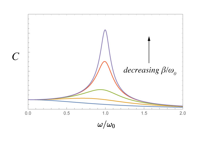
If we decrease the damping (and keep $\omega_0$ constant), we can see the peak of the resonance increasing.
This graph shows 5 different damped driven oscillators. The differences in each curve is the ratio of the damping constant to the resonant frequency. Notice the change in shape.
Quality Factor

The Full Width Half Max measures describes the shape of the curve.

The Quality Factor is the ratio of the resonant frequency, $\omega_0$, and the damping $\beta$.
\begin{equation} Q = \frac{\omega_0}{2 \beta} \end{equation}Applications
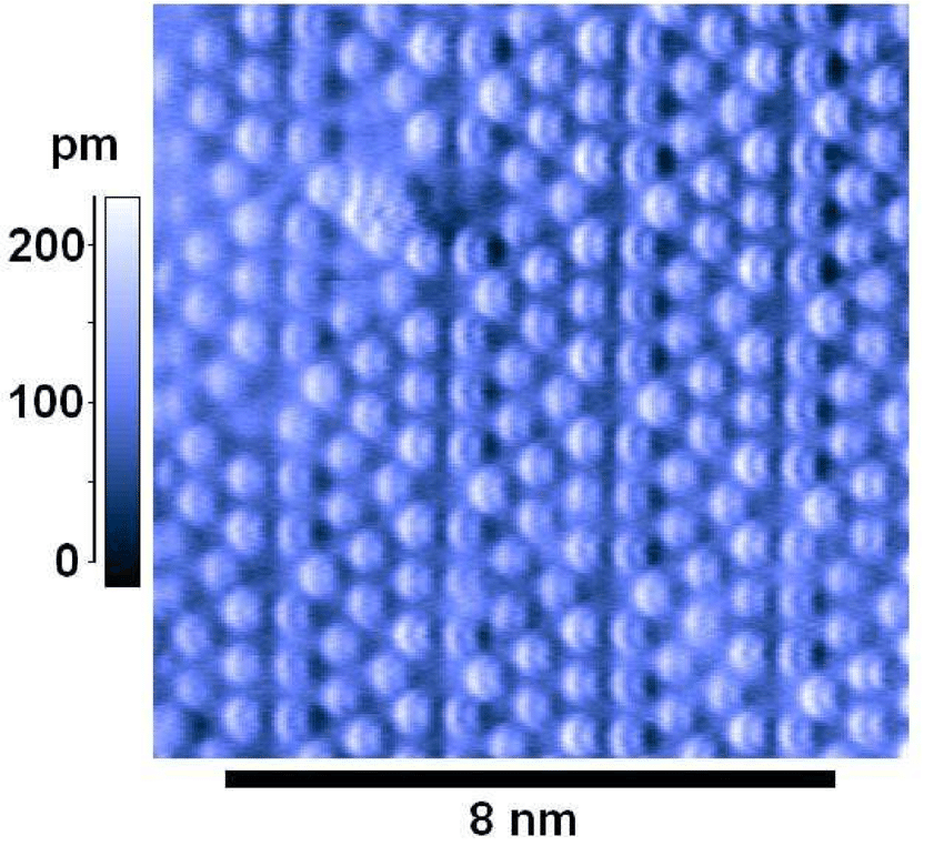
What is this?