Phase Plots
SHO - no damping
\begin{align} x(t) & = A \cos (\omega_0 t + \phi) \\ \dot{x}(t) & = -A \omega_0 \sin (\omega_0 t + \phi) \end{align}Eliminate $t$ and express as a function of ($x$, $\dot{x}$)
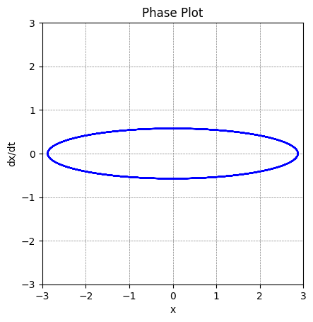
A $x$ vs $\dot{x}$ plot (aka. phase space plot) for a simple harmonic oscillator
The plot is an ellipse, as we'd expect.
The paths never intersect.
Once we have one point, the rest are determined. (i.e. only one trajectory in phase space for a given set of initial conditions)
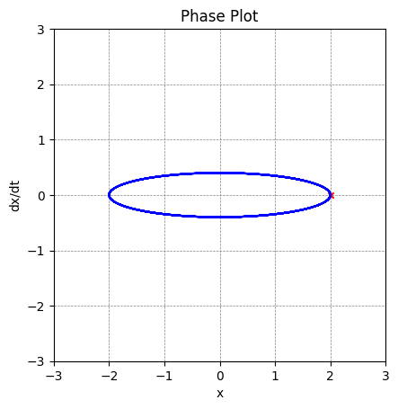
A $x$ vs $\dot{x}$ plot with the initial position and velocity indicated.
Since $A = 2$ and $\phi = 0$ for this plot, we can locate the initial position easily.
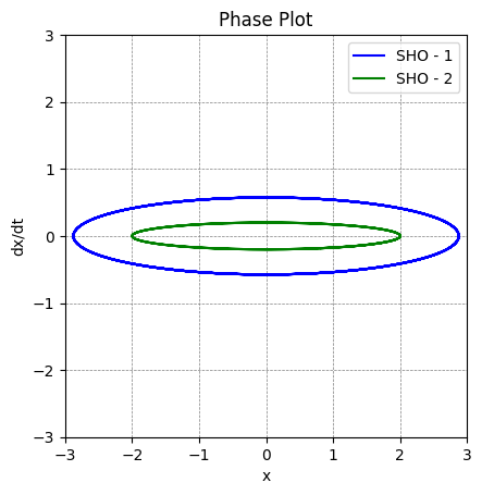
Two $x$ vs $\dot{x}$ plots for a simple harmonic oscillators with different parameters/p>
Changing the parameters like $A$ and $\omega$ will lead to a different ellipse. However, they will all be close trajectories since energy is conserved here.
with: $E = \frac{1}{2}kA^2$ and $\omega_0^2 = \frac{k}{m}$: \begin{equation} \frac{x^2}{2E / k} + \frac{\dot{x}^2}{2 E / m} =1 \end{equation}
\begin{equation} \frac{1}{2}k x^2 + \frac{1}{2} m \dot{x}^2 = KE + PE = E \end{equation}
import numpy as np
import matplotlib.pyplot as plt

x = []
xdot = []
time = np.arange(0,200,.01)

for t in time:
  x.append(A*np.cos(omega0*t))
  xdot.append(-A*omega0*np.sin(omega0*t))

fig, ax = plt.subplots()
ax.plot(x,xdot, label="SHO", color="blue")
ax.scatter(x[0],xdot[0],s=20,c='red',marker='x')
ax.set(xlabel='x', ylabel='dx/dt', title='Phase Plot')
ax.grid(color = 'gray', linestyle = '--', linewidth = 0.5)
ax.set_aspect('equal')
#ax.legend()
ax.set_ylim(-3,3)
ax.set_xlim(-3,3)
plt.show()
With damping?
x = []
xdot = []
x0 = 2
v0 = .3
m = 1
alpha = .1
tau = 2*m/alpha
omega0 = .4
omega1 = np.sqrt(omega0**2-(1/tau**2))
A = np.sqrt(x0**2+((x0+v0*tau)**2/(omega1**2 * tau**2)))
phi = np.arctan(-(x0+v0*tau)/(x0*omega1*tau))
for t in time:

  position = A*np.exp(-t/tau)*np.cos(omega1*t+phi)
  velocity = -A*(1/tau)*np.exp(-t/tau)*np.cos(omega1*t+phi) - A*np.exp(-t/tau)*np.sin(omega1*t+phi)*omega1
  x.append(position)
  xdot.append(velocity)
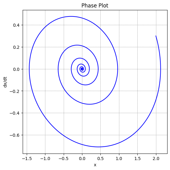
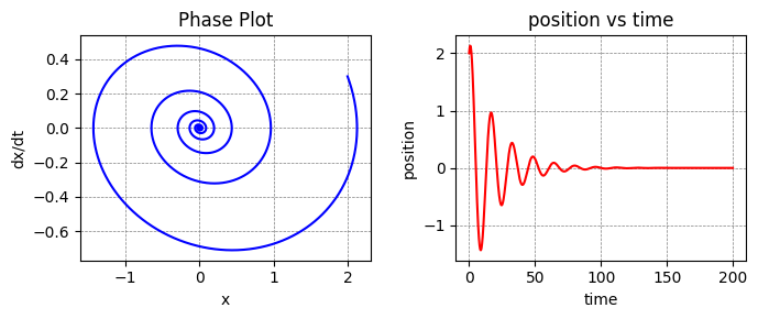
The phase space plot of a damped oscillator.
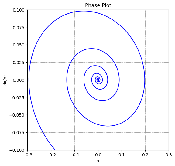
Zoom in to the atractor
  fig, axs = plt.subplots(1, 2, figsize=(7, 3))
  axs[0].plot(x,xdot, label="SHO", color="blue")
  axs[0].set(xlabel='x', ylabel='dx/dt', title='Phase Plot')
  axs[0].grid(color = 'gray', linestyle = '--', linewidth = 0.5)

  axs[1].plot(time,x, label="SHO", color="red")
  axs[1].set(xlabel='time', ylabel='x', title='position vs time')
  axs[1].grid(color = 'gray', linestyle = '--', linewidth = 0.5)
  #ax.set_aspect('equal')
  #ax.legend()
  fig.tight_layout()
  plt.show()
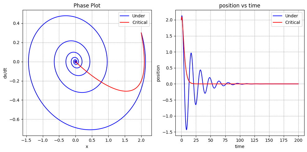
Underdamped and critically damped in the same plot.