Coordinates

Cartesian Coordinates

The Cartesian Coordinate system

The cartesian 3d coordinate system

There are several common ways to express a location:

\begin{align} \mathbf{a} & = a_x \hat{\bf{x}} + a_y \hat{\bf{y}} + a_z \hat{\bf{z}}\\ & = a_x \hat{\bf{i}} + a_y \hat{\bf{j}} + a_z \hat{\bf{k}}\\ & = (a_x,a_y,a_z) \\ & = a_1 \mathbf{e}_1 + a_2 \mathbf{e}_2 + a_3 \mathbf{e}_3 \\ & = \sum_{i=1}^3 a_i \bf{e}_i \\ & = \begin{bmatrix} x_1 \\ x_2 \\ x_3 \end{bmatrix} \end{align}

Vector Math

Magnitudes

$a^2 + b^2 = c^2$

Addition & Subtraction

$$\mathbf{a} = a_1 \hat{\bf{x}} + a_2 \hat{\bf{y}} +a_3 \hat{\bf{z}} $$ And $$\mathbf{b} = b_1 \hat{\bf{x}} + b_2 \hat{\bf{y}} +b_3 \hat{\bf{z}} $$ then, $$\mathbf{a} + \mathbf{b} = (a_1+b_1) \hat{\bf{x}} + (a_2+b_2) \hat{\bf{y}} + (a_3+b_3) \hat{\bf{z}}$$ and $$\mathbf{a} - \mathbf{b} = (a_1-b_1) \hat{\bf{x}} + (a_2-b_2) \hat{\bf{y}} + (a_3-b_3) \hat{\bf{z}}$$

Dot Product

There are two ways of multiplying vectors:

1. The dot product (or scalar product)

$\mathbf{a} \cdot \mathbf{b} = a b \cos \theta$

$\mathbf{a} \cdot \mathbf{b} = (a_1 \hat{\mathbf{x}}+a_2 \hat{\mathbf{y}}+a_3 \hat{\mathbf{z}})\cdot(b_1 \hat{\mathbf{x}}+b_2 \hat{\mathbf{y}}+b_3 \hat{\mathbf{z}}) $

$\mathbf{a} \cdot \mathbf{b} = a_1 b_1 + a_2 b_2 + a_3 b_3$

Dot Product - Linear Algebra

$$ \begin{bmatrix} a_1 \; a_2 \; a_3 \end{bmatrix} \cdot \begin{bmatrix} b_1 \\ b_2 \\ b_3 \end{bmatrix} = a_1 b_1 + a_2 b_2 + a_3 b_3 $$

Cross Product

Defined as: $$\mathbf {a} \times \mathbf {b} =|\mathbf {a} | \; |\mathbf {b}|\; \sin(\theta )\ \mathbf {n} $$ where $\theta$ is the angle between $\mathbf {a} $ and $\mathbf {b}$, and $\mathbf {n}$ is the unit vector perpendicular to the plane containing $\mathbf {a} $ and $\mathbf {b}$

This produces a third vector that points perpendicular to both the original vectors.

$\mathbf{a} \times \mathbf{b} = (a_x \hat{\mathbf{x}}+a_y \hat{\mathbf{y}}+a_z \hat{\mathbf{z}})\times(b_x \hat{\mathbf{x}}+b_y \hat{\mathbf{y}}+b_z \hat{\mathbf{z}}) $

We can calculate the cross product by computing the determinant of this matrix: $$\mathbf{a} \times \mathbf{b} = \begin{vmatrix} \mathbf{\hat{x}} & \mathbf{\hat{y}} & \mathbf{\hat{z}} \\ a_x & a_y & a_z \\ b_x & b_y &b_z \\ \end{vmatrix} $$

$$\mathbf{a} \times \mathbf{b} = (a_y b_z-a_z b_y)\hat{\mathbf{x}}+(a_z b_x-a_x b_z)\hat{\mathbf{y}}+(a_x b_y-a_y b_x)\hat{\mathbf{z}} $$

Mathematica:


    a = {a1, a2, a3}
    b = {b1, b2, b3}
    Dot[a,b]
    -> a1 b1 + a2 b2 + a3 b3
    Cross[a,b]
    -> {-a3 b2 + a2 b3, a3 b1 - a1 b3, -a2 b1 + a1 b2}

numpy (python)


    import numpy as np

    a = np.array([2,4,5])
    b = np.array([1,-2,3])
    c = np.dot(a,b)
    print(c)
    -> 9
    d = np.cross(a,b)
    print(d)
    -> [22 -1 -8]

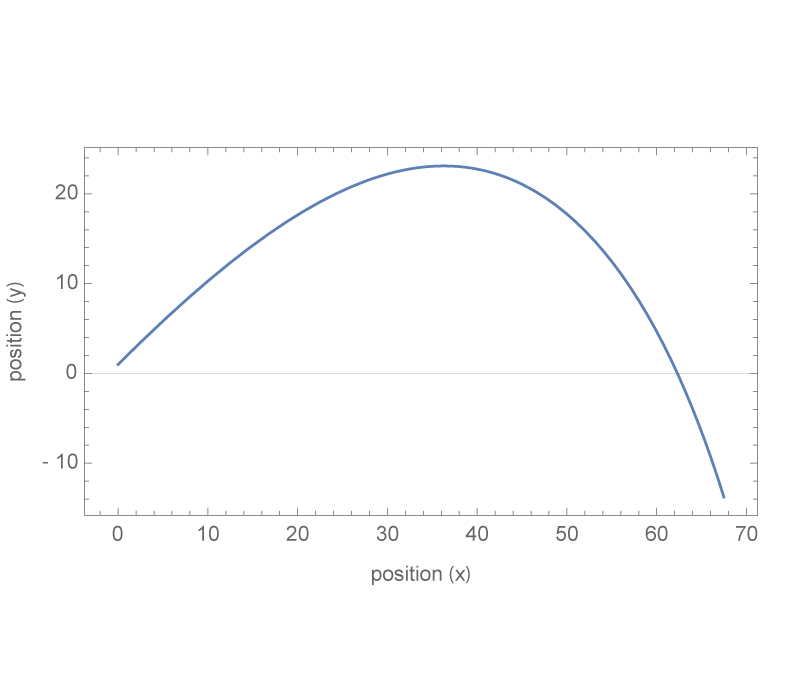
Quadratic Drag in two dimensions

In cartesian coordinates: $$ \begin{align} m \ddot{\mathbf{r}} & = m \mathbf{g} - c v^2 \; \hat{\bf{v}} \\ & = m \mathbf{g} - c v \; \mathbf{v} \end{align} $$

Plot motion for a projectile experiencing quadratic drag.

Mathematica:

Define some parameters


      r = .05;
      area = Pi r^2;
      m = .15;
      g = 9.8;
      Cd = 0.47;
      \[Rho] = 1.29;
      c = 1/2 \[Rho] area Cd;
      \[Theta] = Pi/4
      v0 = 40;

Define our differential equations

In the x direction: $$ m \ddot{x} = -c \dot{x} \sqrt{\dot{x}^2+\dot{y}^2} $$ And $$ m \ddot{y} =-m g -c \dot{y} \sqrt{\dot{x}^2+\dot{y}^2} $$


      diffeqs = {m x''[t] == -c x'[t]*Sqrt[x'[t]^2 + y'[t]^2],
        m y''[t] == -m g - c y'[t]*Sqrt[x'[t]^2 + y'[t]^2],
        x[0] == 0,
        x'[0] == v0 Cos[\[Theta]],
        y[0] == 1,
        y'[0] == v0 Sin[\[Theta]]
        }

Use NDSolve[] to solve them.


      solutions = NDSolve[diffeqs, {x[t], y[t]}, {t, 0, 6}]

Plot x vs. y using ParametricPlot[]


      ParametricPlot[{x[t] /. solutions[[1, 1]], y[t] /. solutions[[1, 2]]}, {t, 0, 5}]

Other Coordinate systems

Polar

The basic polar coordinate system

$$\begin{eqnarray} x &=& r \cos \theta \\ y &=& r \sin \theta \nonumber \\ \end{eqnarray}$$ $$\begin{eqnarray} r = \sqrt{x^2 + y^2} \\ \theta = \tan^{-1} \left(\frac{y}{x}\right) \nonumber \\ \end{eqnarray}$$

Goal: Express newton's laws in these non-cartesian coordinates: $$ F = m\ddot{\mathbf{r}}$$

Unit vectors in polar coordinates

$\mathbf{\hat{r}}$ points in the direction of increasing $r$ (given a fixed $\theta$)

$\boldsymbol{\hat{\theta}}$ points in the direction of increasing $\theta$ (given a fixed $r$)

Now, the unit vectors change!

We start with $\hat{\bf{r}}$

$$ \begin{align} \Delta \hat{\bf{r}}\ & \approx \Delta \theta \; \hat{\boldsymbol{\theta}} \\ & \approx \dot{\theta} \Delta t \; \hat{\boldsymbol{\theta}} \end{align} $$

Taking the time derivative: $$ \frac{d \hat{\bf{r}}}{dt} = \dot{\theta} \; \hat{\boldsymbol{\theta}} $$

Taking the time derivative of $\mathbf{r} = r \hat{\bf{r}}$ \begin{equation} \dot{\mathbf{r}} = \dot{r} \hat{\bf{r}} + r \frac{d \hat{\bf{r}}}{dt} \end{equation} which can be used to express the velocity of the particle in polar coordinates: \begin{equation} \mathbf{v} \equiv \dot{\mathbf{r}} = \dot{r} \hat{\bf{r}} + r \dot{\theta} \; \hat{\boldsymbol{\theta}} \end{equation}

This might look a little different, but you've seen it before. The components are: $$ \begin{align} v_r & = \dot{r}\\ v_\theta & = r \dot{\theta} = r \omega \label{eq:rotationalvelocitycircularmotion} \end{align} $$ \eqref{eq:rotationalvelocitycircularmotion} is just what we had for Uniform Circular Motion, i.e. when $r$ wasn't changing. Now we have to account for changing $r$ values, so we really need both terms.

Velocity expressed in polar coordinates: \begin{equation} \dot{\mathbf{r}} = \dot{r} \hat{\bf{r}} + r \dot{\theta} \; \hat{\boldsymbol{\theta}} \end{equation}

Now we need to get the acceleration

To find the acceleration, we know have to take the time derivative of the velocity: \begin{equation} \mathbf{a} \equiv \ddot{\mathbf{r}} = \frac{d}{dt} \dot{\mathbf{r}} = \frac{d}{dt}\left( \dot{r} \hat{\bf{r}} + r \dot{\theta} \; \hat{\boldsymbol{\theta}} \right) \end{equation}

The new term to deal with is $$ \frac{d \hat{\boldsymbol{\theta}}}{dt} $$ which by similar arguments as above, we can see will be: \begin{equation} \frac{d \hat{\boldsymbol{\theta}}}{dt} = - \dot{\theta} \hat{\bf{r}} \end{equation} Add this back into our acceleration equation: \begin{equation} \mathbf{a} = \left( \ddot{r} \hat{\bf{r}} + \dot{r} \frac{d\hat{\bf{r}}}{dt} \right) + \left( \left( \dot{r} \dot{\theta} + r \ddot{\theta} \right) \hat{\boldsymbol{\theta}} + r \dot{\theta} \frac{d \hat{\boldsymbol{\theta}}}{dt} \right) \end{equation}

Acceleration in polar coordinates: \begin{equation} \mathbf{a} = \left( \ddot{r} - r \dot{\theta}^2 \right)\hat{\bf{r}} + \left( r \ddot{\theta} + 2 \dot{r}\dot{\theta} \right)\hat{\boldsymbol{\theta}} \end{equation}

Example

A mass $m$ is spun around in a circle of radius $R$ at angular velocity $\omega$. Using Newton's 2nd law in polar coordinates, find the tension in the string. No other forces are present.