Accelerating Frames
What do we do if we happen to be in a non-inertial frame?
Linearly Accelerating Frame

a) A ball thrown sideways with an initial velocity $v_0$ in a non-accelerating ship/frame. b) the same trajectory from inside the accelerating ship. c) the same trajectory from out side the accelerating ship.
Inertial Observer

The external observer sees no acceleration in the motion of the ball

The observer in the ship sees something very different.
Let $\mathbf{r}$ be the position in the inertial (external) frame, and $\mathbf{r}'$ in the ship (non-inertial) frame. These can be related through the acceleration of the ship w.r.t the external frame: $a_s$: \begin{equation} \mathbf{r} = \mathbf{r}' + \frac{1}{2}\mathbf{a}_s t^2 \end{equation}
Velocities are likewise found to be (through differentiation w.r.t $t$): \begin{equation} \mathbf{v} = \mathbf{v}' + \mathbf{a}_s t \end{equation} and acceleration: \begin{equation} \mathbf{a} = \mathbf{a}' + \mathbf{a}_s \end{equation}

The non-inertial observer sees a new force: $\mathbf{F}'$
In the inertial frame: $\mathbf{F} = m \mathbf{a}$, or, considering the two frames: \begin{equation} \mathbf{F} = m \mathbf{a} = m \left(\mathbf{a}' + \mathbf{a}_s \right) \end{equation} or, considering a new $\mathbf{F}'$: \begin{equation} \mathbf{F}' = m \mathbf{a}' = \mathbf{F} - m \mathbf{a}_s \end{equation}
So, for observers inside the non-inertial frame: \begin{equation} \mathbf{F}' = \mathbf{F} + \mathbf{F}_\textrm{pseudo} \end{equation}
This observed force, $\mathbf{F}'$ is the sum of any real forces and the Pseudo-Forces created by the accelerating reference frame.
Example: effective gravity for the accelerating ship: \begin{equation} \mathbf{F} = 0 \end{equation} but \begin{equation} \mathbf{F}' \neq 0 = 0 - m \mathbf{a}_s = m \mathbf{a}' \end{equation} thus: \begin{equation} \mathbf{a}' = -\mathbf{a}_s \end{equation}
In this simple case, we can call our pseudo-force, the effective gravity: \begin{equation} \mathbf{g}_\textrm{eff} = - \mathbf{a}_s \end{equation} Everything can be done that same as before if we include this in our set-up.
What about the Lagrangian approach? \begin{equation} L = T' - U' \end{equation} where $T'$ is the kinetic energy in the non-inertial frame, and $U'$ would include and pseudo-potentials: \begin{equation} L = \frac{1}{2}m \left( \dot{x}'^2 + \dot{y}'^2 \right) - m g_\textrm{eff} y' \end{equation}
The pendulum in an accelerating frame

A pendulum in an accelerating spacecraft
Find the Lagrangian for the non-inertial observer:
\begin{equation} L = T' - U' = \frac{1}{2}m R^2 \dot{\theta}'^2 - m g_\textrm{eff} R \left(1 - \cos \theta' \right) \end{equation}
Rotating Frames

A vector in a rotating frame
Assume vector $\mathbf{A}$ is at rest in the rotating frame. As the frame rotates, the vector $\mathbf{A}$ will also rotate through an angle $d \phi$. The change in $\mathbf{A}$ can then be expressed by the cross-product: \begin{equation} d\mathbf{A} = d \boldsymbol{\phi} \times \mathbf{A} \end{equation}
($d \boldsymbol{\phi}$ points out of the page)
Now, what if $\mathbf{A}$ is also changing in the rotating frame? \begin{equation} d \mathbf{A}_\textrm{in} = d \mathbf{A}_\textrm{rot} + d \boldsymbol{\phi} \times \mathbf{A} \end{equation}
Next, consider the time derivatives: \begin{equation} \left. \frac{d \mathbf{A}}{dt} \right|_\textrm{in} = \left. \frac{d \mathbf{A}}{dt} \right|_\textrm{rot} + \boldsymbol{\omega} \times \mathbf{A} \end{equation} where $\omega = \frac{d\phi}{dt}$
Helpful to consider this an operator: \begin{equation} \left. \frac{d}{dt} \right|_\textrm{in} = \left. \frac{d }{dt} \right|_\textrm{rot} + \boldsymbol{\omega} \times \end{equation} This can operate on any vector and will transform from one coordinate system to another: inertial -> rotating.
Now we express the velocity in the inertial frame in terms of the velocity in the rotating frame (let our position be $\mathbf{r}$): \begin{equation} \mathbf{v}_\textrm{in} = \mathbf{v}_\textrm{rot} + \boldsymbol{\omega} \times \mathbf{r} \end{equation}
Using this, we can construct the Lagrangian: \begin{equation} L = \frac{1}{2}m \mathbf{v}^2 - U(\mathbf{r}) \end{equation}
Now for some vector math: $$ \begin{aligned} \frac{1}{2}m \left(\mathbf{v}_\textrm{rot} + \boldsymbol{\omega} \times \mathbf{r} \right)^2 = & \frac{1}{2}m \mathbf{v}_\textrm{rot}^2 + m \mathbf{v}_\textrm{rot} \cdot \left( \boldsymbol \omega \times \mathbf{r} \right) + \frac{1}{2}m \left( \boldsymbol \omega \times \mathbf{r}\right)^2 \\ = & \frac{1}{2}m \mathbf{v}_\textrm{rot}^2 + m \mathbf{v}_\textrm{rot} \cdot \left(\boldsymbol \omega \times \mathbf{r} \right) + \frac{1}{2}m \omega^2 r^2 - \frac{1}{2}m \left( \boldsymbol \omega \cdot \mathbf{r} \right)^2 \end{aligned} $$
Thus, in the rotating frame, were we to construct a Lagrangian based on our measurements, we would obtain: \begin{equation} L = \frac{1}{2}m \mathbf{v}_\textrm{rot}^2 + m \mathbf{v}_\textrm{rot} \cdot \left(\boldsymbol \omega \times \mathbf{r} \right) + \frac{1}{2}m \omega^2 r^2 - \frac{1}{2}m \left( \boldsymbol \omega \cdot \mathbf{r} \right)^2 - U(\mathbf{r}) \end{equation} This is clearly not just $\frac{1}{2}m \mathbf{v}_\textrm{rot}^2$
Find the equations of motion using the Lagrangian: \begin{equation} \frac{d}{dt}\left( \frac{\partial L}{\partial \dot{r}_\textrm{rot}^i} \right) = \frac{\partial L}{\partial r_\textrm{rot}^i} \end{equation}
Here, $i$ implies $x$, $y$, and $z$ in the rotating frame.
\begin{equation} L = \frac{1}{2}m \mathbf{v}_\textrm{rot}^2 + m \mathbf{v}_\textrm{rot} \cdot \left(\boldsymbol \omega \times \mathbf{r} \right) + \frac{1}{2}m \omega^2 r^2 - \frac{1}{2}m \left( \boldsymbol \omega \cdot \mathbf{r} \right)^2 - U(\mathbf{r}) \end{equation}
So, taking the time derivative of $\frac{\partial L}{\partial \dot{r}_\textrm{rot}^i}$: \begin{equation} \frac{d}{dt}\left( \frac{\partial L}{\partial \dot{r}_\textrm{rot}^i} \right) = m \ddot{r}_\textrm{rot}^i + m \left(\boldsymbol{\omega} \times \mathbf{v}_\textrm{rot} \right)^i + m \left( \frac{d \boldsymbol{\omega}}{dt } \times \mathbf{r} \right)^i \end{equation}
\begin{equation} L = \frac{1}{2}m \mathbf{v}_\textrm{rot}^2 + m \mathbf{v}_\textrm{rot} \cdot \left(\boldsymbol \omega \times \mathbf{r} \right) + \frac{1}{2}m \omega^2 r^2 - \frac{1}{2}m \left( \boldsymbol \omega \cdot \mathbf{r} \right)^2 - U(\mathbf{r}) \end{equation}
For the R.H.S. ($\frac{\partial L}{\partial r_\textrm{rot}^i}$): first rewrite one term as: \begin{equation} m \mathbf{v}_\textrm{rot} \cdot \left( \boldsymbol{\omega} \times \mathbf{r} \right) = m \mathbf{r} \cdot \left(\mathbf{v}_\textrm{rot} \times \boldsymbol{\omega} \right) \end{equation}
Now the Lagrangian is: \begin{equation} L = \frac{1}{2}m \mathbf{v}_\textrm{rot}^2 +m \mathbf{r} \cdot \left(\mathbf{v}_\textrm{rot} \times \boldsymbol{\omega} \right) + \frac{1}{2}m \omega^2 r^2 - \frac{1}{2}m \left( \boldsymbol \omega \cdot \mathbf{r} \right)^2 - U(\mathbf{r}) \end{equation}
\begin{equation} L = \frac{1}{2}m \mathbf{v}_\textrm{rot}^2 +m \mathbf{r} \cdot \left(\mathbf{v}_\textrm{rot} \times \boldsymbol{\omega} \right) + \frac{1}{2}m \omega^2 r^2 - \frac{1}{2}m \left( \boldsymbol \omega \cdot \mathbf{r} \right)^2 - U(\mathbf{r}) \end{equation}
Leads to: \begin{equation} \frac{\partial L }{\partial r_\textrm{rot}^i} = m \left( \mathbf{v}_\textrm{rot} \times \boldsymbol{\omega} \right)_\textrm{rot}^i + m \omega^2 r_\textrm{rot}^i - m \left( \boldsymbol{\omega} \cdot \mathbf{r} \right)\omega^i - \frac{\partial U(\mathbf{r})}{\partial r_\textrm{rot}^i} \end{equation}
Thus our equation of motion in the rotating system is: \begin{equation} m \mathbf{a} = m \omega^2 \mathbf{r}_\textrm{rot} - m \left( \boldsymbol{\omega} \cdot \mathbf{r} \right) \boldsymbol{\omega}_\textrm{rot} - 2 m \left( \boldsymbol{\omega} \times \mathbf{v}_\textrm{rot} \right)_\textrm{rot} - m \left( \frac{d\boldsymbol{\omega}}{dt} \times \mathbf{r} \right)_\textrm{rot} - \nabla_\textrm{rot} U(\mathbf{r}) \end{equation}
Combine the first two terms: \begin{equation} m \omega^2 \mathbf{r}_\textrm{rot} - m \left( \boldsymbol{\omega} \cdot \mathbf{r} \right) \boldsymbol{\omega}_\textrm{rot} = -m \boldsymbol{\omega} \times \left( \boldsymbol{\omega } \times \mathbf{r} \right)_\textrm{rot} \end{equation} (using a vector identity.)
Finaaaaly, \begin{equation} \mathbf{F}_\textrm{rot} = \mathbf{F}_\textrm{in} -m \boldsymbol{\omega} \times \left( \boldsymbol{\omega } \times \mathbf{r} \right)_\textrm{rot} - 2 m \left( \boldsymbol{\omega} \times \mathbf{v}_\textrm{rot} \right)_\textrm{rot} - m \left( \dot{\boldsymbol{\omega}} \times \mathbf{r} \right)_\textrm{rot} \end{equation} where $\mathbf{F}_\textrm{in} = - \nabla_\textrm{rot} U(\mathbf{r})$ is the sum of real forces acting in the inertial frame
What are these pseudo-forces?, \begin{equation} \mathbf{F}_\textrm{rot} = \mathbf{F}_\textrm{in}\; \underbrace{- m \boldsymbol{\omega} \times \left( \boldsymbol{\omega } \times \mathbf{r} \right)_\textrm{rot} }_\textrm{centrifugal}\; \underbrace{- 2 m \left( \boldsymbol{\omega} \times \mathbf{v}_\textrm{rot} \right)_\textrm{rot}}_\textrm{Coriolis} \; \underbrace{- m \left( \dot{\boldsymbol{\omega}} \times \mathbf{r} \right)_\textrm{rot}}_\textrm{Euler} \end{equation}
Pseudo-Forces
Centrifugal
\begin{equation} - m \boldsymbol{\omega} \times \left( \boldsymbol{\omega } \times \mathbf{r} \right)_\textrm{rot} \end{equation}

Verify the direction of the centrifugal pseudo-force
Coriolis
\begin{equation} - 2 m \left( \boldsymbol{\omega} \times \mathbf{v}_\textrm{rot} \right) \end{equation}
The Coriolis force acts when the object is moving in a direction that is not parallel to $\boldsymbol{\omega}$
Euler
\begin{equation} - m \left( \boldsymbol{\dot{\omega}} \times \mathbf{r} \right)_\textrm{rot} \end{equation}
This pseudo-force only arises when $\omega$ is changing, i.e. the speed of rotation is changing.
Earth as rotating reference frame
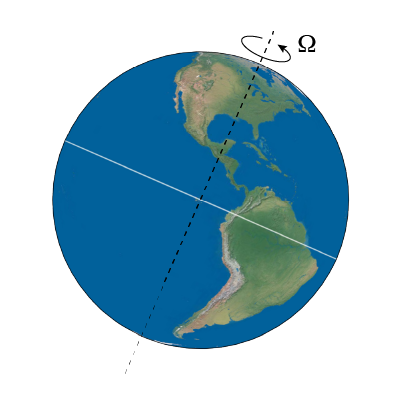
The Earth Rotating on its axis
Earth takes 24 hours to rotate once.
(Actually, a little bit less: sidereal day is 23h56'04'') $$ \begin{aligned} \Omega & = \frac{2\pi}{24 \; \textrm{h} \times 3600 \; \textrm{s/h}} \left(\frac{366.5}{365.5} \right) \\ & = 7.292 \times 10^{-5} \; \textrm{s}^{-1} \end{aligned} $$
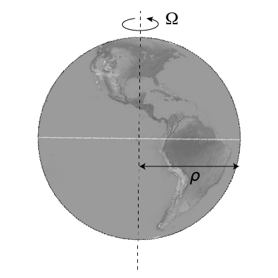
Let $\rho$ be the distance from the rotation axis.
The Centrifugal pseudo-force will be directed outward and proportional to the distance from the rotation axis $\rho$. \begin{equation} \mathbf{F}_\textrm{cent} = - m \boldsymbol{\omega} \times \left( \boldsymbol{\omega } \times \mathbf{r} \right)_\textrm{rot} \end{equation} can be simplified to: \begin{equation} F = m \Omega^2 \rho \end{equation} Taking the radius at the equator to be 6378 km: \begin{equation} 6.374 \times 10^{6} \; \textrm{m} \times \left( 7.292 \times 10^{-5} \; \textrm{s}^{-1}\right)^2 = 0.033914 \; \textrm{m}/\textrm{s}^2 \end{equation} Which is about 0.3% of the normal $g$.
Thus, the effective gravity would be: \begin{equation} g_\textrm{eff} = g - \Omega^2 \rho \end{equation} The value of $\rho$ depends on latitude, and you can easily see how at the poles, this contribution should be zero.
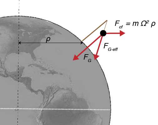
Forces on a plumb bob in the northern hemisphere
Since these are all vectors, we can see the effects on a plumb-bob hanging in the north hemisphere: \begin{equation} \mathbf{F}_\textrm{G-eff} = \mathbf{F}_G - \mathbf{F}_\textrm{cf} \end{equation}
Coriolis
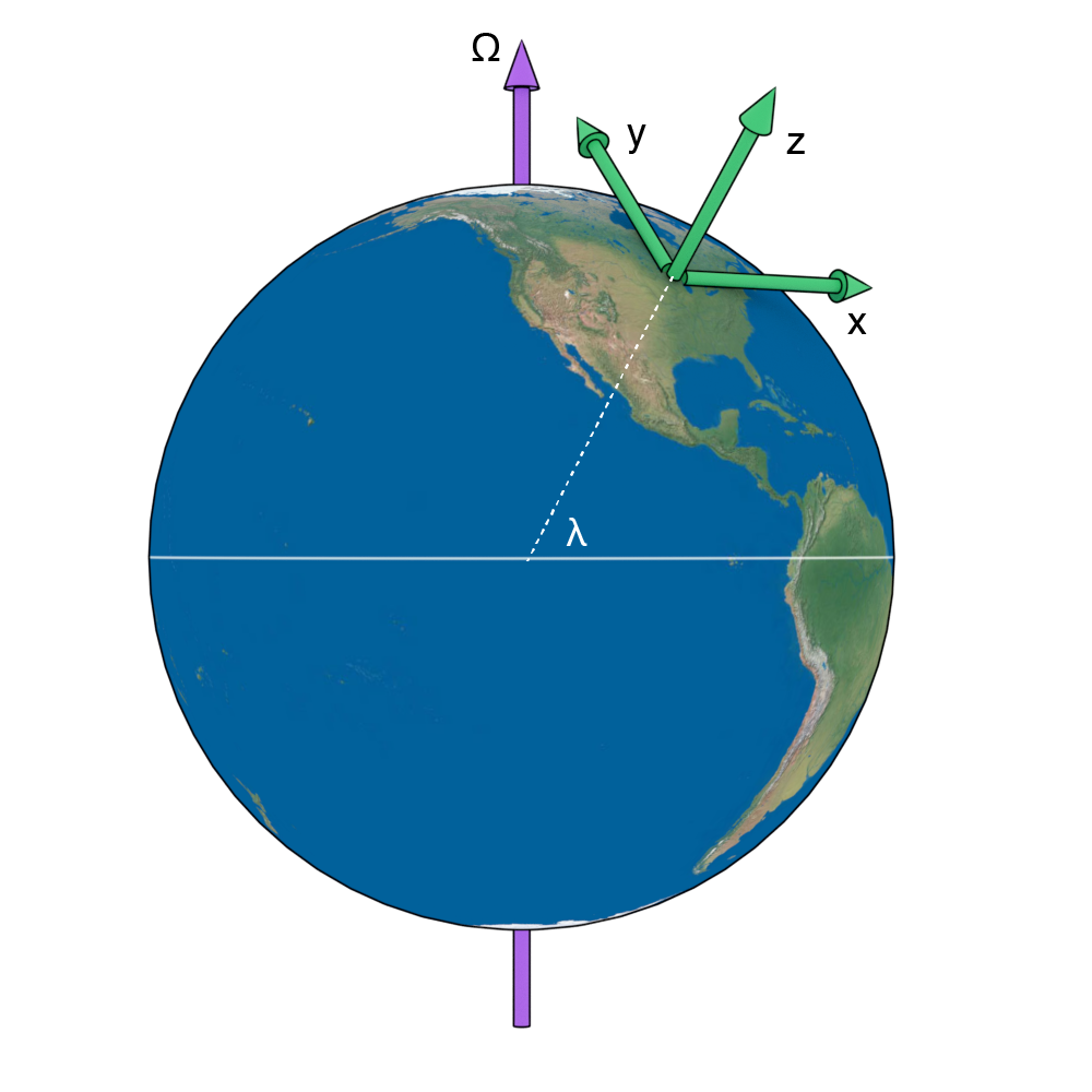
A cartesian set on the surface of the Earth.
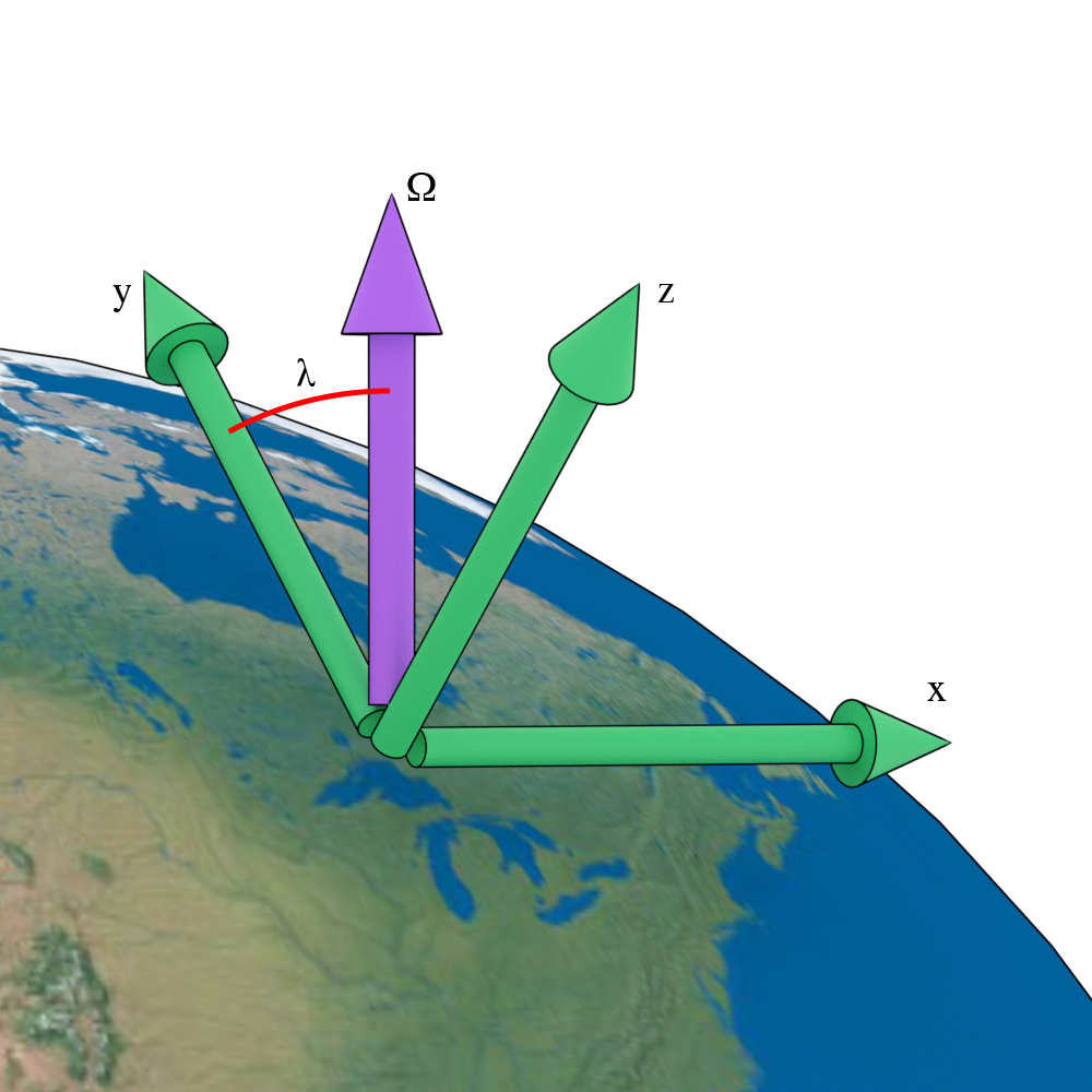
A cartesian set on the surface of the Earth.
Express $\Omega$ in terms of cartesian vectors: \begin{equation} \boldsymbol{\Omega} = \Omega \left(\hat{\bf{y}} \cos \lambda + \hat{\bf{z}} \sin \lambda \right) \end{equation}
A particle will have velocity components: \begin{equation} \mathbf{v} = \dot{x} \hat{\bf{x}} + \dot{y} \hat{\bf{y}} + \dot{z} \hat{\bf{z}} \end{equation}
Thus we can compute the Coriolis pseudo-force vector: $$ \begin{align} \mathbf{F}_\textrm{Cor} & = -2 m \boldsymbol{\Omega} \times \mathbf{v} \\ & = 2 m \Omega \left[ \left( \dot{y} \sin \lambda - \dot{z} \cos \lambda \right) \hat{\bf{x}} - \dot{x} \sin \lambda \; \hat{\bf{y}} + \dot{x} \cos \lambda \; \hat{\bf{z}}\right] \end{align} $$
If there is no vertical motion, i.e. $\dot{z} = 0$: \begin{equation} \mathbf{F}_\textrm{Cor, horiz} = 2 m \Omega \sin \lambda \left( \dot{y} \hat{\bf{x}} - \dot{x} \hat{\bf{y}} \right) \end{equation} but $\mathbf{v} = (\dot{x},\dot{y}) = \left( v \cos \theta, v \sin \theta \right)$ so: \begin{equation} \mathbf{F}_\textrm{Cor, horiz} = 2 m \Omega \sin \lambda v \left( \sin \theta \hat{\bf{x}} - \cos \theta \hat{\bf{y}} \right) \end{equation}

The $\mathbf{r}$ and $\mathbf{v}$ and $\boldsymbol{\theta}$ vectors
or, in terms of the vector: $\hat{\boldsymbol{\theta}}$ \begin{equation} \mathbf{F}_\textrm{Cor, horiz} = -2 m \Omega \sin \lambda v \hat{\boldsymbol{\theta}} \end{equation}
- The Coriolis force therefore pushes moving objects the right of their velocity vector if $\sin \lambda \gt 0$ (i.e. northern hemisphere)
- The Coriolis force therefore pushes moving objects the left of their velocity vector if $\sin \lambda \lt 0$ (i.e. southern hemisphere)
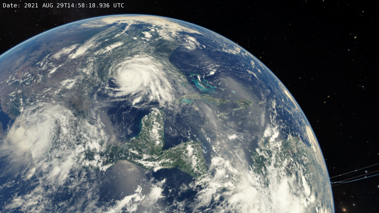
Hurricane Ida
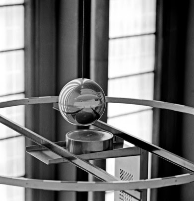
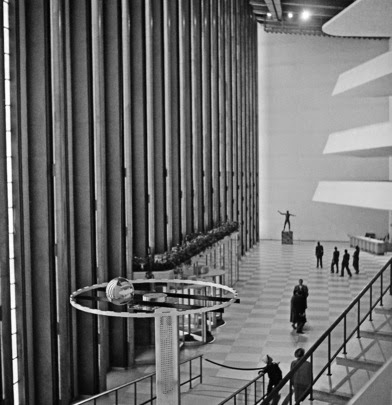
Foucault Pendulum
The forces in the rotating frame of the Earth: \begin{equation} m \ddot{\mathbf{r}} = \mathbf{T} + m \mathbf{g}_0 + m \left(\boldsymbol{\Omega} \times \mathbf{r} \right) \times \boldsymbol{\Omega} + 2 m \dot{\mathbf{r}} \times \boldsymbol{\Omega} \end{equation}
Combine $\mathbf{g}_0$ and $m \left(\boldsymbol{\Omega} \times \mathbf{r} \right) \times \boldsymbol{\Omega}$ to express in terms of the observed gravitational force: \begin{equation} m \ddot{\mathbf{r}} = \mathbf{T} + m \mathbf{g} + 2 m \dot{\mathbf{r}} \times \boldsymbol{\Omega} \end{equation}

The Pendulum
As usual, let's restrict ourselves to small oscillations
This let's us say that \begin{equation} T \approx mg \end{equation} since $T_z = T \cos \beta \approx T$
Next, we need to examine the x and y components
Looking at the figure: \begin{equation} \frac{T_x}{T} = -\frac{x}{L} \;\; \textrm{and} \;\; \frac{T_y}{T} = -\frac{y}{L} \end{equation} therefore: \begin{equation} T_x = \frac{-mgx}{L} \;\; \textrm{and} \;\; T_y = \frac{-mgy}{L} \end{equation}
\begin{equation} m \ddot{\mathbf{r}} = \mathbf{T} + m \mathbf{g} + 2 m \dot{\mathbf{r}} \times \boldsymbol{\Omega} \end{equation}
Then we have two equations of motion, after some algebra $$ \begin{align} \ddot{x} & = \frac{-gx}{L} + 2 \dot{y} \Omega \cos \theta \\ \ddot{y} & = \frac{-gy}{L} - 2 \dot{x} \Omega \cos \theta \end{align} $$
$\theta$ is the colatitude of the experiment.
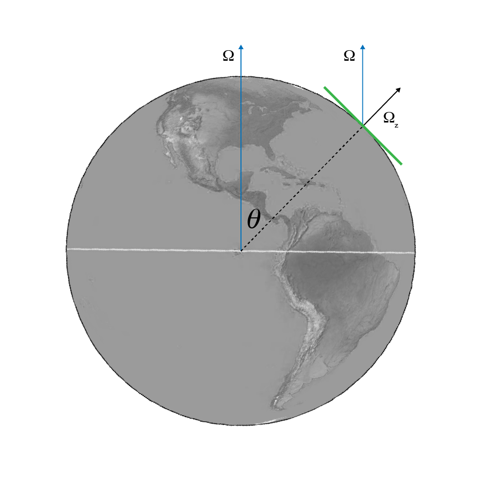
The $\Omega_z$ and colatitude angle $\theta$.
A little more cleaning up and we have: $$ \begin{align} \ddot{x} - 2 \dot{y} \Omega_z + \omega_0^2 x = 0 \\ \ddot{y} + 2 \dot{x} \Omega_z + \omega_0^2 y = 0 \\ \end{align} $$
Let's solve these. $$ \begin{align} \ddot{x} - 2 \dot{y} \Omega_z + \omega_0^2 x = 0 \\ \ddot{y} + 2 \dot{x} \Omega_z + \omega_0^2 y = 0 \\ \end{align} $$
Start by defining a complex number: \begin{equation} \eta = x + iy \end{equation} And multiply the $\ddot{y}$ equation by $i$, then add it to the $\ddot{x}$ equation: \begin{equation} \ddot{\eta} + 2 i \Omega_z \dot{\eta} + \omega_0^2 \eta = 0 \end{equation}
Now we have a second-order, linear, homogeneous differential equation.
This implies two indepedent solutions
Try: $\eta(t) = e^{-i\alpha t}$
Leads to: \begin{equation} \alpha^2 - 2 \Omega_z \alpha - \omega_0^2 = 0 \end{equation} or \begin{equation} \alpha = \Omega_z \pm \sqrt{\Omega_z^2+ \omega_0^2} \end{equation}
Thus: \begin{equation} \eta = e^{-i\Omega_z t}\left(C_1 e^{i \omega_0 t} + C_2 e^{-i \omega_0 t} \right) \end{equation}
With $x = A$ and $y = 0$ at $t = 0$, the pendulum is released from rest ($v_{x0} = v_{y0} = 0$) and we can obtain: \begin{equation} C_1 = C_2 = \frac{A}{2} \end{equation}
\begin{eqnarray} \eta(t) & = & x(t) + iy(t) \\ & = & A e^{-i \Omega_z t} \cos \omega_0 t \end{eqnarray}