Gauss's Law
Introductory Analogies

Consider these two diagrams of flowing air.
We can think about the amount of air passing through each of the two loops. Intuitively, we would expect that amount is greater in the upper section.
Let's try to quantify that difference
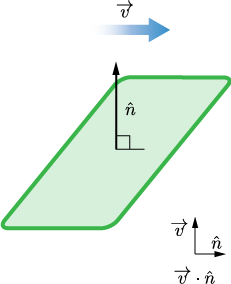
We must first define a unit vector perpendicular to the surface: $\hat{n}$.
The vector field can be described by a vector $\overrightarrow{v}$.
If we want to determine how perpendicular these vectors are in relation to each other, we can take the dot product of the two:
$$\overrightarrow{v} \cdot \hat{n} = |v||n|\cos \theta$$
Which of the following could be the surface normal unit vector at the point where the red dot is located?
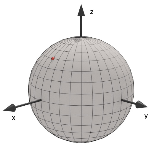
- $\langle \frac{1}{\sqrt{3}},\frac{1}{\sqrt{3}},\frac{1}{\sqrt{3}} \rangle$
- $\langle \frac{1}{\sqrt{2}},0,\frac{1}{\sqrt{2}} \rangle$
- $\langle 1,0,1 \rangle$
- $\langle 0,1,0 \rangle$
- $\langle -1,-1,1 \rangle$

Thus, in these two cases, we can see by comparing the dot products of the two vectors that the amount of flow through the loop should be drastically different depending on its rotation:
Upper: $\overrightarrow{v}\cdot \hat{n} = vn\cos(0^\circ) = vn$
Lower: $\overrightarrow{v}\cdot \hat{n} = vn\cos(90^\circ) = 0$
And any angle in between can be accounted for in a similar manner.
What quantity from 207 involved calculating a dot product?
- Kinetic Energy
- Momentum
- Work
- Torque
- Temperature
Vector $\overrightarrow{P}$ extends from point < 0,0,0 > to point < 2, 6, 7>. What is the dot product of $\overrightarrow{P}$ and the surface normal for the plane, $\mathbf{\hat{n}}$? (i.e. find $\overrightarrow{P} \cdot \mathbf{\hat{n}} $ )
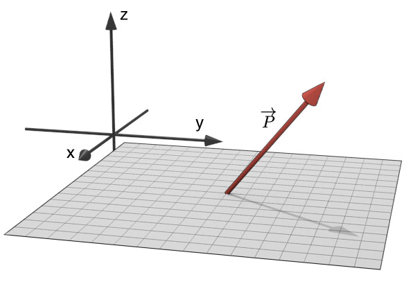
- 0
- 1
- 15
- 7
- 9.4
Which of these vectors has the smallest dot product with the surface normal?

Flow to field
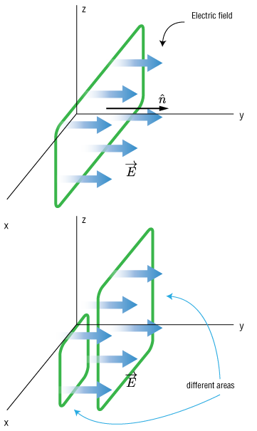
Of course, Electric fields are a bit different than flowing air, however, we can use the same mathematical framework to describe them.
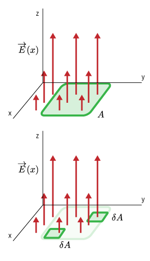
Another aspect we'll need to account for, in addition the angle of the surface we're dealing with, is its area.
Again, it should be intuitive that for a uniform field like the one shown, if we consider a larger area, the amount of 'flow' through the surface should be larger.
And so, our measure for the amount field passing through a given surface of area $A$ can be written: $$\overrightarrow{E}\cdot \overrightarrow{A} = EA\cos \theta$$ ($\overrightarrow{A}$ is a vector with a magnitude given by the area, and the direction given by the normal of its surface.)
We'll call this quantity flux.
In particular, when talking about electric fields, we'll use the term Electric Flux, and give it the symbol $\Phi_e$.
For a constant electric field, we can say the flux through an area, $A$, is given by
$$\bbox[10px,border:3px solid red]{\Phi_e = \overrightarrow{E}\cdot \overrightarrow{A}}$$Multiple Surfaces

Without too much stress, we could imagine adding up several of the planes.
Each plane would have its own normal vector, given by its area. It wouldn't be too much trouble to figure out the flux through each one, and then add them together.
$$\Phi_e = \Phi_e^1 +\Phi_e^2 +\Phi_e^3 +\Phi_e^4 =\sum_i^4 \Phi_e^i$$.Flux is a scalar quantity, so the values found will just add using scalar arithmetic.
One closed surface

And finally, we'll need to be comfortable with the notion of a closed surface. This is just an assemblage of smaller surfaces, each with the own normal vector and area.
In the case shown, we have a cube shape which is enclosed by six squares.
Uniform Field?
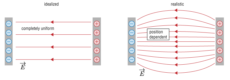
Have we ever really had a completely uniform electric field? Nope. Our capacitor model required that the two plates be infinitely large, as well as closely spaced. This can work in the land of abstractions, but not in the real world.
So, we should be prepared to deal with non-uniform fields as well.
Fortunately, a little calculus will solve this problem. Instead of considering one large area $A$, we can break $A$ up into smaller sections, $\delta A$. Thus, each little square will have a litle flux passing through it:
$$\delta \Phi_i = \overrightarrow{E}_i \cdot \delta \overrightarrow{A}_i$$To find the total flux through our original area $A$, we'll just need to add up all the little areas:
$$\Phi_e = \sum_i \overrightarrow{E}_i \cdot \delta \overrightarrow{A}_i$$ In the limit $\delta \overrightarrow{A} \rightarrow d\overrightarrow{A}$, we can make this an integral: $$\Phi_e = \int \overrightarrow{E} \cdot d\overrightarrow{A}$$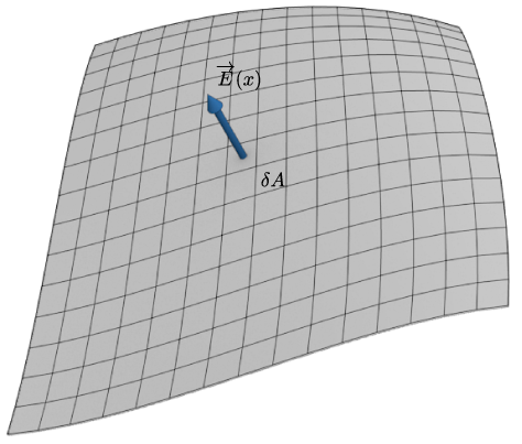
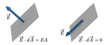
If we have both a spatially dependent $\overrightarrow{E}$, and a surface that is not flat, then we have to be a little more careful about this process. One aspect that makes things easier, is the realization that if an $\overrightarrow{E}$ vector is tangent to a surface element, then the flux will be zero, and if it is perpendicular, then $\Phi_e = EA$.
Close it up
Finally, we'll add on last piece of math notation. That's the surface integral
It's just a little circle in the integral sign which means we have to perform the integration over a closed surface.
$$\int \Rightarrow \oint$$.What have we done so far?
$$\Phi_e = \oint \overrightarrow{E} \cdot d \overrightarrow{A}$$What can we do with this?
If we have a given function for $\overrightarrow{E}$, then we can figure out the flux by evaluating the integral. We can't really do it very easily for any arbitrary surface, so we'll have to chose out integration surfaces wisely.
In the context of electric fields, we'll call the surfaces Gaussian Surfaces. They aren't real, material surfaces, but mathematical constructs.
Symmetry
Normally, when we think of the word symmetry, we think of a situation like this:

Here is an idealized butterfly, and it's symmetric about the vertical axis. Meaning, we can mirror it about an axis aligned through the vertical direction, and we can't tell the new one from the old one.
Symmetry
However, that is just one of many ways an object can be symmetric.
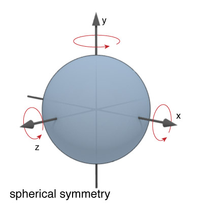
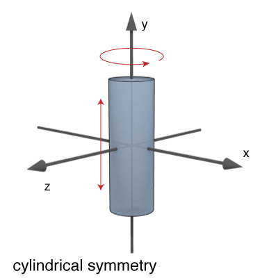

Three different types of symmetry: spherical, cylindrical, and planar.
Infinite vs. Finite
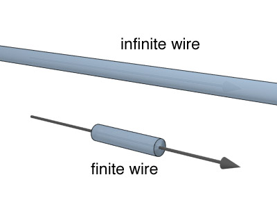
Planar and cylindrical symmetry really only exists for infinite planes or cylinders. In the case of a finite cylinder, there are of course two ends. If we were walking along the cylinder, and we got to an end, we would certainly be notice something different.
However, if we were only asking about a very small section of the cylinder, that was very far from the ends, then we might not notice that there were ends to the cylinder, in which case, the cylinder is effectively infinite according to our perspective.
Infinite vs. Finite
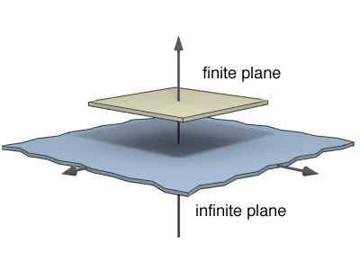
The same is true of the plane. Only if we are very small, and far from the edges, does the plane seem infinite to us.
Electrostatics Implications
Question: What does this have to do with electrostatics?
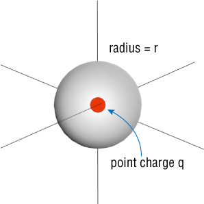
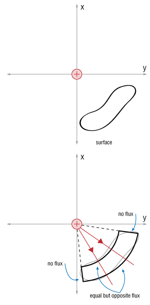
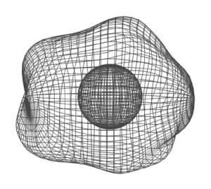
We'll put a point charge $q$ at the origin. Then we'll enclose it in a sphere with radius r.
Just by inspection, since the field from a point charge is radially directed, we can figure out the flux integral to be:
$$\Phi_e = \oint \overrightarrow{E} \cdot d \overrightarrow{A} = EA_\textrm{sphere}$$where $A_\textrm{sphere}$ is the area of the sphere given by: $4 \pi r^2$
We also know Coulomb's law for the electric field from a point charge:
$$E = \frac{q}{4 \pi \epsilon_0 r^2}$$Answer: Everything!
Thus our Flux through the sphere is equal to
$$\Phi_e = \frac{q}{4 \pi \epsilon_0 r^2} (4 \pi r^2) = \frac{q}{\epsilon_0}$$where $q$ is the point charge at the origin.
What would the flux be for a sphere with a radius equal to 4 times that in the previous problem, i.e. it contains a charge $q$ and has a radius $=4r$?
- $\Phi_e = 4q/\epsilon_0$
- $\Phi_e = q/ 4\epsilon_0$
- $\Phi_e = q/ \epsilon_0$
- $\Phi_e = q/16 \epsilon_0$
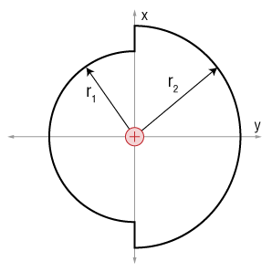
We'll do the same thing, but this time for a 'weird sphere' like this one.
Considering the left side first, we'll find that the flux through that surface, the smaller hemisphere, will give:
$$\Phi_1 = \oint \overrightarrow{E} \cdot d \overrightarrow{A} = \frac{q}{2 \epsilon_0}$$Likewise, the right hemisphere, despite its larger radius still has the same flux:
$$\Phi_2 = \oint \overrightarrow{E} \cdot d \overrightarrow{A} = \frac{q}{2 \epsilon_0}$$And the two sections along the $x$ axis will contribute nothing to the total flux, because they are parallel to the field lines.
Thus, the total flux through this surface is:
$$\Phi_e = \Phi_1+\Phi_2 = \frac{q}{\epsilon_0}$$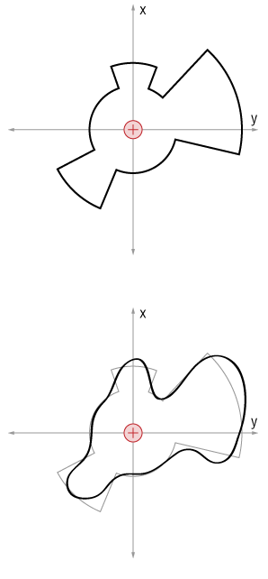
In fact, any surface made of radial and spherical pieces will have the same flux:
$$\Phi_e = \frac{q}{\epsilon_0}.$$And, since we can approximate any shaped surface by a collection of radial and spherical pieces, in the limit, then we say that any closed surface surrounding the point charge $q$ will have the same flux!
$$\Phi_e = \oint \overrightarrow{E} \cdot d\overrightarrow{A} =\frac{q}{\epsilon_O}$$This result might seem shocking, but it's really a consequence of the inverse square law.
Consider the four situations shown. Each one contains either a charge $q$ or a charge $2q$. Each case shows a Gaussian surface surrounding a point charge. Considering the electric flux $\Phi$ through each of the Gaussian surfaces, which of the following comparative statements is correct?
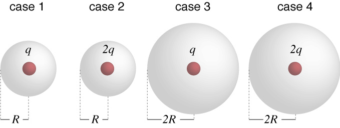
- $\Phi_1 = \Phi_3 > \Phi_2 = \Phi_4$
- $\Phi_1 = \Phi_4 > \Phi_2 = \Phi_3$
- $\Phi_2 = \Phi_4 > \Phi_1 = \Phi_3$
- $\Phi_2 > \Phi_1 > \Phi_4 > \Phi_3$
- $\Phi_3 = \Phi_4 > \Phi_2 = \Phi_3$
What will happen if the charge is out side our Gaussian surface?
We can use the same formulation, and by approximating any arbitrary surface as a set of spherical and radial surfaces, we can see that again, the radially directed components won't contribute (zero flux through them), but the spherical sections will have non-zero flux values. However, they will be equal and opposite, since the fields are parallel to one surface, and anti-parallel to the other. Thus, the net electric flux through closed surface is zero, if that surface does not contain a charge.
What about more than one charge?

Since we can add fields, we can find the total flux by summing the contributions from each individual charge:
$$\Phi_e = \oint \overrightarrow{E}_1 \cdot d\overrightarrow{A}+\oint \overrightarrow{E}_2 \cdot d\overrightarrow{A}+\ldots $$ $$\Phi_e = \Phi_1 + \Phi_2 \dots $$And therefore, the total flux for the distribution of charges inside an arbitrary closed surface will just be the sum of the individual contributions.
$$\Phi_e = \frac{q_1}{\epsilon_0}+\frac{q_2}{\epsilon_0}+\ldots$$We can add all these charges together to get a total charge enclosed: $Q$.
$$Q = q_1+q_2+\ldots$$Positive and Negative
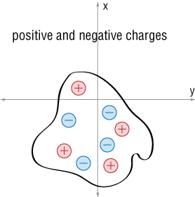
And, if we have both negative and positive charges, we can account for that by considering the sign of the $\overrightarrow{E}$ in the flux equation. A positive $\overrightarrow{E}$ will be considered an outward flux, while the field from a negative charge will be an inward flux.
Gauss's Law
And, we are back to the beginning, with what we will call Gauss's law:
$$\boxed{\Phi_e = \oint \overrightarrow{E} \cdot d\overrightarrow{A} =\frac{Q}{\epsilon_O}}$$
In words, the net flux through a surface is equal to the charge enclosed.
How can we use this?
By carefully selecting a sensible Gaussian surface around a known charge distribution, we can calculate electric fields that would have been difficult to do so using Coulomb's Law.
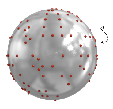
An amount of charge $q$ is spread evenly over the surface of this hollow metal sphere of radius $R$. Find the electric field profile starting from the center of the sphere.
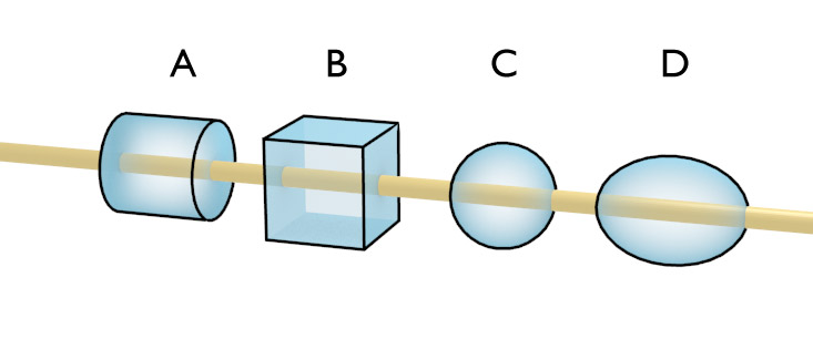
Which of the four shapes would be a good Gaussian Surface to find the field from a charged wire?
Examples of Gauss' Law
Field from a line charge

$$E = \frac{\lambda}{2 \pi \epsilon_0 r}$$
Field from a plane of charge
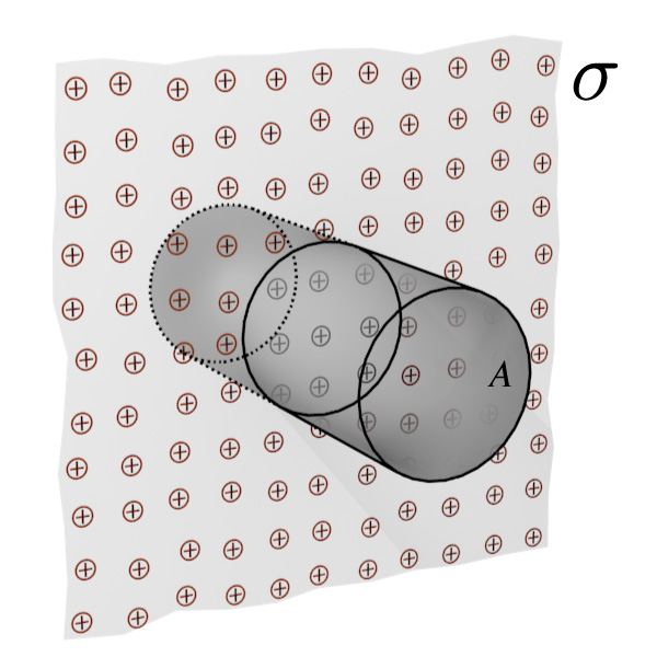
$$E = \frac{\sigma}{2\epsilon_0}$$
Two conducting planes
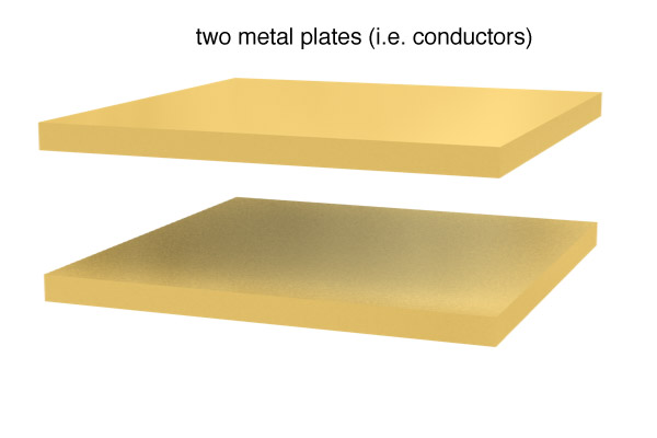
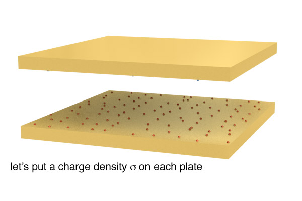


Let's start by considering the field from one plate.
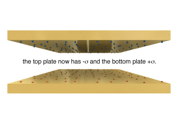
$$E = \frac{\sigma}{2 \epsilon_0}$$Likewise a second plate with opposite charges on it will have the same field, also pointed in the same direction:
$$E = \frac{\sigma}{2 \epsilon_0}$$Together, these fields will add to create a uniform field given by:
$$E = \frac{\sigma}{ \epsilon_0}$$
Parallel Plate Capacitor
This configuration will be called a parallel plate capacitor.
For now, we'll use this configuration to create a uniform field. In the future we'll use it many more contexts.
Where is the charge?
Since charges in the presence of an electric field will be accelerated, we can use the converse of this to state that if charges are stationary, then there is no net electric field.

Thus, we expect that within a conducting body in equilibrium, i.e. where no charges are moving, there should be no net electric fields.
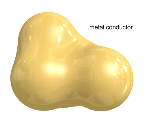
Conductors and Charge
Looking inside a charged conductor
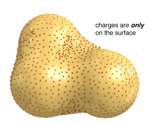
The charge on a conductor will be on the surface.

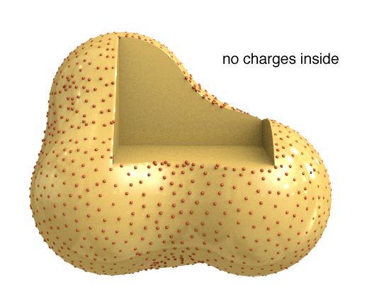
Let's take a conductor and carve out a cavity from the inside.
Visualizing a slice of this new shape might look like this:


Faraday Cage
Inside two plates, we'll have a uniform field.


However, a conducting box placed within the field will not have a field inside of it.

Fields at the surface of a conductor


If a conductor becomes charged, it will no doubt be the source of an electric field.
If the conductor is in equilibrium, i.e. no moving charges, then the field directions must be perpendicular to the surface.
If they were not, then they would cause surface charges to accelerate.
Gauss' law in spherical systems
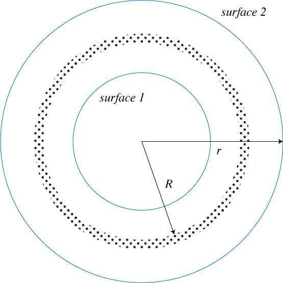
Imagine a spherical shell of radius $R$ and charge $q$. Assume the charge is distributed uniformly. We can take two Gaussian surfaces and find very different results.
For a Gaussian surface with $r \geq R$:
$$E = \frac{1}{4\pi\epsilon_0}\frac{q}{r^2}$$If we take a Gaussian surface inside the shell however, then Gauss's law will tell us that:
$$ E = 0$$Gauss' law in spherical systems

Now, for a solid sphere of charge, we have a different situation.
If our gaussian surface is within the sphere of charge:
$$E = \frac{1}{4 \pi \epsilon_0}\frac{qr}{R^3}$$And if outside:
$$E = \frac{1}{4 \pi \epsilon_0} \frac{q}{r^2}$$Which plot would best describe the electric field strength as a function of position for a charged, conducting sphere with radius R, centered at the origin?

Gauss Law Summary
- $\bbox[10px,border:2px solid black]{\Phi =\oint \overrightarrow{E} \cdot d\overrightarrow{A} = \frac{q_\textrm{enc}}{\epsilon_0}}$
- Excess charge on a conductor is located entirely on the outer surface.
- The electric field near the surface of a charged conductor is perpendicular to the surface.
- There are no electric fields within the conductor
An infinite slab of charge of thickness $2a$ is centered in the $xy$ plane. The charge density is $$\rho = \rho_0 \left( 1-\frac{|z|}{a} \right).$$ Find the electric fields strengths inside and outside the slab.