Potential, the electric kind
Potential Energy

A spring is compressed by doing work. In the process, its potential energy is increased.
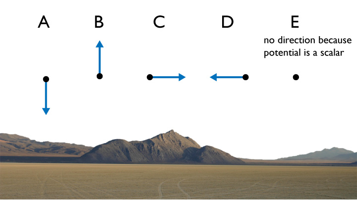
What’s the direction of the gravitational potential energy of a 2kg ball 10 meters above the ground?


Moving charges closer to the source charges will require more work.

Test charges charges will have large forces acting, and thus will require more work to move them.

Another situation might involve moving different amounts of charge in an electric field.
These charges have different q’s. So, again, it take more work to bring the more heavily charged object closer to the source charges.
Electric Potential
Let's introduce a new concept: The Electric Potential, $V$.

The Electric Potential V at various positions.
We’ll call it V. It has the units of Joules/Coulomb, aka volts.
$$\bbox[10px,border:2px solid red]{U = q_0 V}$$
The zero potential
Just like in determining the gravitational potential energy, we were free to pick where we wanted the $U = 0$ point to be.
Usually it was the ground, but it could have also been the top of a table, or a mountain, etc.
In electrostatics, we'll generally set the $U = 0$ point at infinity.
$$x = \infty \Rightarrow U_\textrm{elec} = 0$$In mechanics, if we applied a constant force over a distance at some angle, we calculated the work like this.
$W = F \Delta x \cos\theta$Then we could find the change in potential energy.
$W = -\Delta U = -(U_f - U_i)$
A charge placed between two charged plated (i.e. a capacitor) will experience a force, and accelerate in a direction determined by the filed.
We can find a constant force inside a capacitor. If we let the field do work on the charge, and move it a distance x, then the work can be found by:
$$ W = q E x = -\Delta U_\textrm{elec}$$Electric Potential Energy
The amount of potential energy, relative to a specified zero, for a particular charge in an electric field. $$\Delta U = - W = -\int \mathbf{F}\cdot d\mathbf{x}$$.
(Units are Joules.
or electronVolts 1 eV = $1.6 \times 10^-19$ J)
Electric Potential
The electric potential is given by the amount of electric potential energy a point charge of 1 Coulomb would have at a given location in space.$$V \equiv \frac{U_\textrm{elec}}{q_0}$$
Units are Volts [V] or Joules/Coulomb.
Simalarly, like the electric field, the electric potential of a charge distribution is defined everywhere in space.
Electric Potential Energy
Let's calculate the potential energy of a two charge system.

Two like charges will repel each other based on Coulomb's law

If object 2 moves from $x_i$ to $x_f$, the electric field will do work:$$W_\textrm{elec} = \int_{x_i}^{x_f} F_\textrm{1 on 2} \;dx$$
$$W_\textrm{elec} = \int_{x_i}^{x_f} F_\textrm{1 on 2} \;dx$$
$$W_\textrm{elec} = \int_{x_i}^{x_f} \frac{1}{4 \pi \epsilon_0} \frac{q_1 q_2}{x^2} dx$$
$$W_\textrm{elec} = \frac{q_1 q_2}{4 \pi \epsilon_0} \left.\frac{-1}{x} \right|_{x_i}^{x_f}$$
$$W_\textrm{elec} = - \frac{q_1 q_2}{4 \pi \epsilon_0}\frac{1}{x_f} + \frac{q_1 q_2}{4 \pi \epsilon_0}\frac{1}{x_i}$$
$$\Delta U = U_f - U_i = -W(i \rightarrow f) = \frac{q_1 q_2}{4 \pi \epsilon_0}\frac{1}{x_f} - \frac{q_1 q_2}{4 \pi \epsilon_0}\frac{1}{x_i}$$
$$U_\textrm{elec} = \frac{q_1 q_2}{4 \pi \epsilon_0}\frac{1}{x}$$
Two examples

A positive particle moving in the direction of the field. $$U_i - U_f > 0$$ (The potential energy has decreased)

A positive particle moving in the direction opposite to the field. $$U_i - U_f < 0$$ (The potential energy has increased)

Since $V = U/q$, we can now figure out a value for $V$ as a function of position within the plates.
$$U_i - U_f = qEx$$$$V_i - V_f = \frac{U_i-U_f}{q} = Ex$$
$$\Delta V_C = V_+ - V_- = Ed$$
$$E = \frac{\Delta V_C}{d}$$
$$V = \frac{x}{d}{\Delta V_C}$$
Graphical Representations

Three representations of a change in potential as a function of position. Left: Potential vs. Position line chart; center: schematic showing geometry of plates (gray) and two equipotential surfaces inside; right) x-y slice showing location of 1 V and 2 V positions.

Is the $\Delta V$ seen (felt) by this particle positive, negative, or zero after it moves from i to f ?

- Positive: $\Delta V > 0 $
- Negative: $\Delta V < 0$
- Zero: $\Delta V = 0$
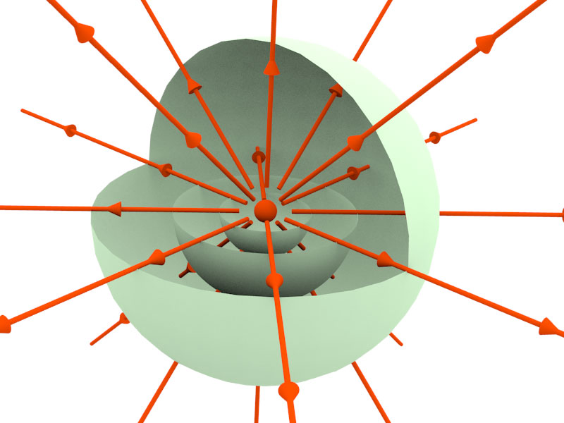
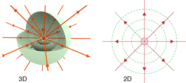
A 3D and 2D representation of equipotential surfaces.
Field Lines and Potential
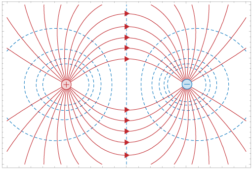
Field lines in red, equipotential surfaces in dotted blue lines.
Calculate the potential from the field
$dW = \mathbf{F} \cdot d\mathbf{s} = q_0 \mathbf{E} \cdot d\mathbf{s}$
$ W = q_0 \int_i^f \mathbf{E} \cdot d\mathbf{s}$
$V_f - V_i = \frac{\Delta U}{q_0} = -\frac{W}{q_0}$
$V_f - V_i = -\int_i^f \mathbf{E} \cdot d\mathbf{s}$
$\bbox[10px ,border:3px solid red]{V = -\int_i^f \mathbf{E} \cdot d\mathbf{s}}$
Find the electric potential distribution in space due to a point charge
Determine if the potential energy of the particle increases, decreases, or stays the same between the initial and final positions.

- Increases
- Decreases
- Stays the same
Determine if the potential energy of the particle increases, decreases, or stays the same between the initial and final positions.

- Increases
- Decreases
- Stays the same
Determine if the potential energy of the particle increases, decreases, or stays the same between the initial and final positions.

- Increases
- Decreases
- Stays the same
Determine if the potential energy of the particle increases, decreases, or stays the same between the initial and final positions.

- Increases
- Decreases
- Stays the same

- Find the potential at points A and B
- Find the potential difference between points A and B
- Find the potential energy of a proton at points A and B
- Find the speed of a proton at point b that was moving to the right at point a with a speed of $4 \times 10^5$ m/s.
- Find the speed of a proton at point a that was moving to the left at point b with a speed of $4 \times 10^5$ m/s.
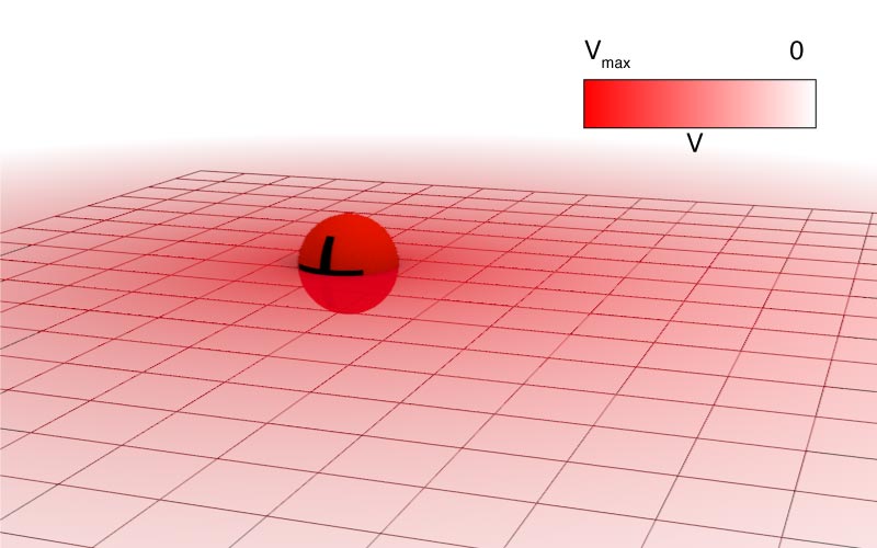
Potential of a point charge
For a point charge with charge $q$, the electric potential is given by:

Plot of electric potential from a point charge as a function of position away.
$$V = \frac{1}{4 \pi \epsilon_0} \frac{q}{r}$$
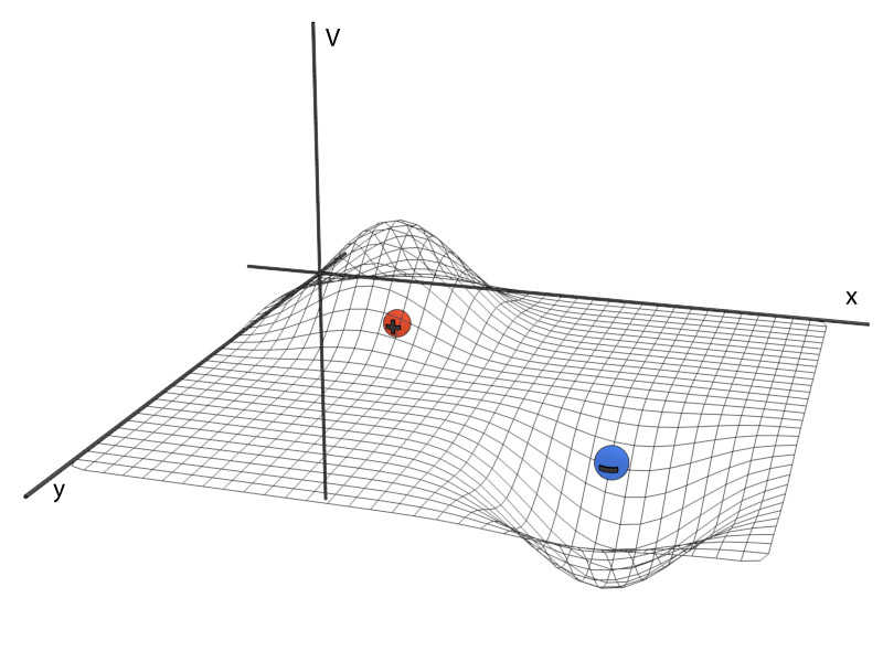
Or, we visualize this as an energy landscape.
Potential from multiple point charges
Since potential is a scalar, we can find the electric potential due to many point charges just by adding each one up:
$$V = \sum_{i= 1}^N V_i = \frac{1}{4 \pi \epsilon_0} \sum_{i= 1}^N \frac{q_i}{r}$$We do need to keep track of the charge, since that will determine the potential sign.

Find the electric potential at point P due to the two charges shown.
The superposition principle

Electric potentials can be added easily since they are scalar quantities.
Potential due to a dipole

Show that the potential due to a dipole can be given by
$$V = \frac{1}{4 \pi \epsilon_0} \frac{p \cos \theta}{r^2}$$Potential due to a continuous charge distribution
$$V = \sum_{i= 1}^N V_i = \frac{1}{4 \pi \epsilon_0} \sum_{i= 1}^N \frac{q_i}{r}$$Was for continuous charges. In this case of a continuous distribution, where we can consider the infinitesimal elements:
$$V = \int dV = \frac{1}{4 \pi \epsilon_0} \int \frac{dq}{r}$$A line of charge
Show that the potential for a line of charge of length $L$ and density $\lambda$ above one end is given by:
$$V = \frac{\lambda}{4 \pi \epsilon_0} \ln \left[ \frac{L + (L^2+d^2)^{1/2}}{d}\right]$$
A disc of charge
Show that the potential for a disc of charge of length $R$ and density $\sigma$ above the central axis at a height $z$ is given by:
$$V = \frac{\sigma}{2 \epsilon_0} (\sqrt{z^2+ R^2}-z)$$
Field from the potential
The work done by a field to move a charged object across an infinitesimal electric potential difference is. $$dW = -q_0 dV$$
We can also calculate the work from the electric field over an infinitesimal distance:
$$dW = q_0 E \cos \theta ds$$
Thus: $$ -q_0 dV = q_0 E \cos \theta ds$$
or: $$E_s = -\frac{\partial V}{\partial s}$$

Field Lines and potential from a point charge
In component form:
$$E_x = -\frac{\partial V}{\partial x}$$ $$E_y = -\frac{\partial V}{\partial y}$$ $$E_z = -\frac{\partial V}{\partial z}$$Direction of the field
The nabla, or del operator:
$$\nabla = \mathbf{\hat{x}} {\partial \over \partial x} + \mathbf{\hat{y}} {\partial \over \partial y} + \mathbf{\hat{z}} {\partial \over \partial z}$$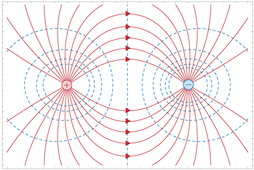
The field is perpendicular to equipotential surfaces!

Below are equipotential lines for an unknown charge distribution. Compare the electric field strength at points a and b.
- The electric field is weaker at point A than point B
- The electric field is stronger at point A than point B
- The electric field is the same at points A and B
- No information about the electric field can be obtained from this graph
Problem
A charge with 5/9 nC is located at the origin.
- Find the positions along the x axis where the potential is 500, 400, 300, 200 and 100 V.
- Plot V(x) for the range: $-10$ cm $< x < +10 $cm.
- Figure out using the slope of the previous graph what the direction of the electric field is to the left and right of the charge.
- Draw a 2d map of the charge (looking down from above) and draw the equipotential lines and some electric field lines.
Below is a graph of the electric potential along the x axis. Two point charges, $q_a$ and $q_b$ are located at points a and b.

- What are the signs of $q_a$ and $q_b$?
- What is the ratio: $|\frac{q_a}{q_b}|$?
- Draw a qualitative graph of the x-component of the electric field, $E_x$, as a function of x, on the axis below.
Potential energy of a system of point charges

We can ask: "What is the potential energy of a system of point charges?"
The answer: "How much work did it cost to build it?
What is the electric potential energy of the following system of charges?

What is the electric potential $U$ of the following system of charges? Let $q_1 = +q$ and $q_2 = -4 q$ and $q_3 = +2q$ where $q = 150 nC$. The distance $d$ is equal to 12 cm.
Potential of a charged conductor

Since: $$\Delta V = -\int_i^f \mathbf{E}\cdot d\mathbf{s},$$ and $$E = 0$$ inside a conductor, we can say that the electric potential everywhere inside a conductor in equilibrium is the same.
Things about conductors
- All excess charge is on the surface,
- The electric field inside is zero,
- The exterior field is perpendicular to the surface,
- The entire conductor is at the same potential.

At which point is the gradient of this hill the highest?
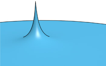
Shape of the conductor matters
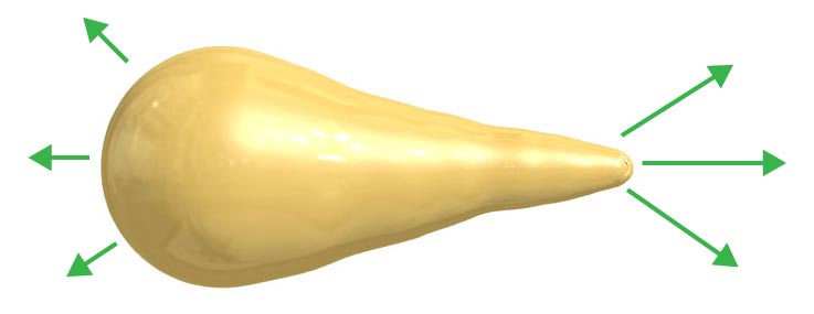
A conductor with regions of differing geometries.
Since $$\mathbf{E} = -\nabla V =-\left( \mathbf{\hat{x}} {\partial V \over \partial x} + \mathbf{\hat{y}} {\partial V \over \partial y} + \mathbf{\hat{z}} {\partial V \over \partial z} \right)$$ we can see that where the potential changes the most as a function of position, the electric fields should be the largest.
Thus, for conductors with pointy parts, the electric field will be the highest in those regions.
Things about conductors
- All excess charge is on the surface,
- The electric field inside is zero,
- The exterior field is perpendicular to the surface,
- The entire conductor is at the same potential.
- The field is strongest at sharp corners