Spectral Lines
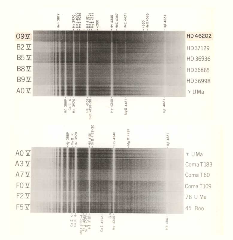
Stellar spectra (negatives) for main-sequence classes O9-F5. (Since the image is a negative, the absorption lines are the bright lines)
H.A. Abt, A.B. Meinel, W.W. Morgan & J.W. Tapscott An Atlas of Low Dispersion Grating Stellar Spectra NSF? 1968
Early spectrometers produced their results on photographic plates. Astronomers would visually inspect the data to analyze the spectra. Figure
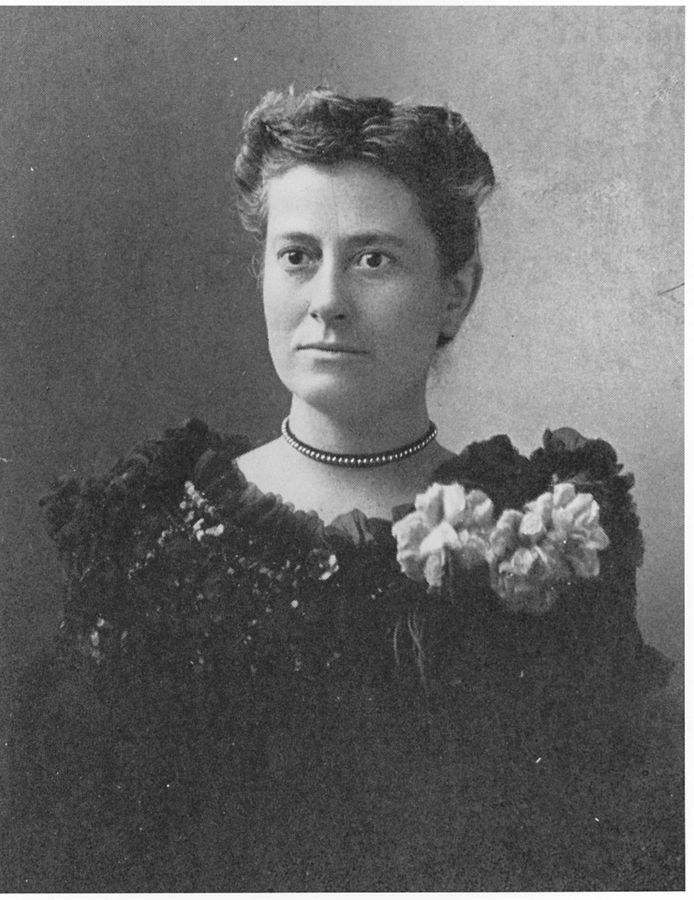
Williamina Stevens
By Unknown - http://www.cfa.harvard.edu/lib/online/almanac/0300c.htm, Public Domain, https://commons.wikimedia.org/w/index.php?curid=9430839
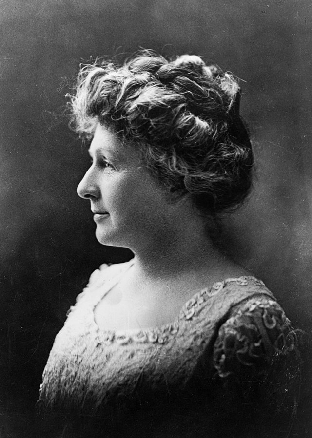
Annie Jump Cannon
By New York World-Telegram and the Sun Newspaper - http://www.britannica.com/EBchecked/topic/92776/Annie-Jump-Cannon, Public Domain, https://commons.wikimedia.org/w/index.php?curid=9431030
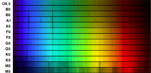
A more modern color spectrum showing the absorption lines from the various classes of stars.
Harvard Spectral Classification
Stellar Classes
Spectral Type Color Characteristics
O Hottest Blue-white Strong He II abs. B Hot Blue-white He 1 abs. strongest at B2 A White Balmer abs. strongest at A0 Ca II abs. stronger F Yellow-white Ca II strengthen Balmer weakens G Yellow Solar Type Spectra Fe I, neutral metal lines stronger K Cool Orange Ca II strongest K0 dominated by metal absorption lines M Cool Red dominated by molecular abs. L Very Cool dark red Metal Hydrides, Water, CO, alkalis T Coolest Infrared Methane (CH4)
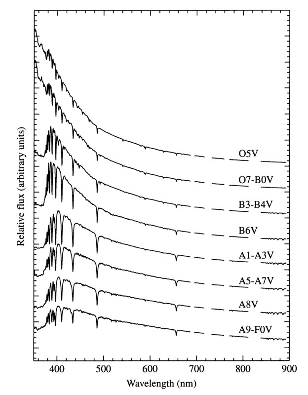
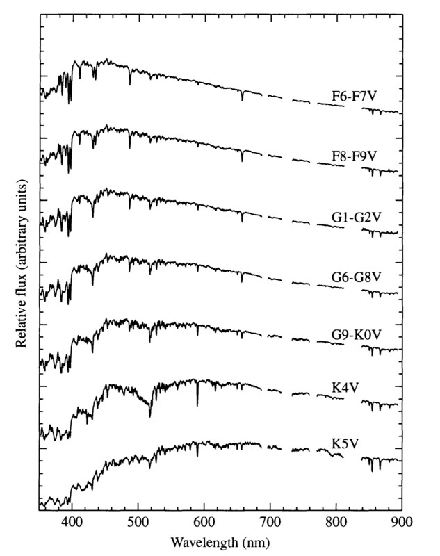
Spectra of main sequence stars
Ap. J. Suppl 81 , 865 1992
Spectra of main sequence stars
Ap. J. Suppl 81 , 865 1992
How are these spectra created?
Now that we understand the basic elements of emission and absorption, we can attempt to sort out what the observed spectra mean in terms of the physics happening inside a star. It will be useful to understand the statistics of the multitude of atom that exist in the stars.
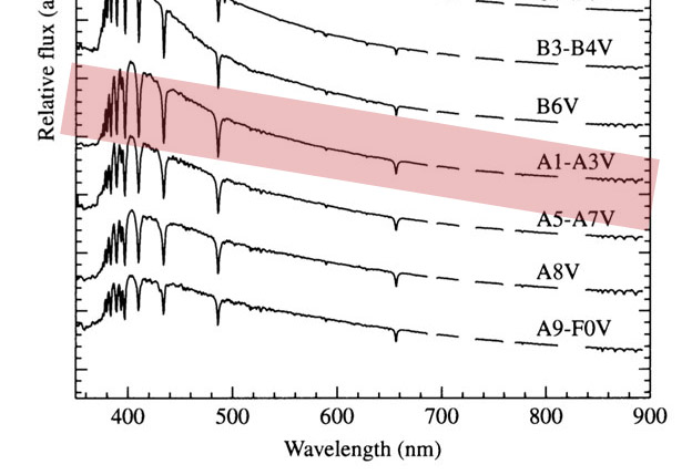
The A0 spectra
The A1 line has the most pronounced Balmer series.
Balmer is strongest. Temp is approximately 10,000 k. Can we understand why?
Balmer Lines
The Balmer series
$$\begin{equation}
\frac{1}{\lambda} = R_H \left( \frac{1}{2^2} - \frac{1}{n^2} \right)
\end{equation}$$
The Boltzmann Distribution
$$\begin{equation}
e^{-\frac{E}{kT}}
\end{equation}$$
The Boltzmann Factor gives the distribution of an energy state $E$, while at a temperature $T$. As $E$ increases, the probably of finding that state decreases.
The Boltzmann Equation
$$\begin{equation}
\frac{N_b}{N_a} = \frac{g_b e^{-E_b / kT}}{g_a e^{-E_a / kT}} = \frac{g_b}{g_a}e^{-(E_b-E_a)/kT}
\label{eq:the-boltzmann-equation}
\end{equation}$$
The Boltzmann equation above, allows us to calculate the ratio of atoms with different energies: $E_b$ and $E_a$. $g_a$ is the degeneracy . For the ground state, there are two configurations with the same energy, so that gives $g = 2$. In general,
$$\begin{equation}
g = 2 n^2
\end{equation}$$
where $n$ is the energy level. (1 is ground state)
Find the temperature of a gas of neutral hydrogen atoms when the gas contains the same amount of ground state (n = 1) and 1st excited state hydrogen atoms.
If the two populations are equal, then the ratios on either side of eq. \eqref{eq:the-boltzmann-equation} will be 1.
$$\begin{equation}
1 = \frac{2(2)^2}{2(1)^2} e^{-[(-13.6 \; \textrm{eV}/2^2)-(-13.6 \; \textrm{eV}/1^2)]/kT}
\end{equation}$$
We can rearrange this to:
$$\begin{equation}
\frac{10.2 \; \textrm{eV}}{kT} = \ln (4)
\end{equation}$$
Solving for $T$:
$$\begin{equation}
T = \frac{10.2 \; \textrm{eV}}{k \ln (4)} = 8.54 \times 10^4 \; \textrm{K}
\end{equation}$$
So, at temperatures above ~85,000 K, half the hydrogen atoms will be in the first excited state.
If the temperature continues to increase, we would expect, based on this analysis, that the number of hydrogen atom in the 1st exited state would continue to increase. Likewise, we would expect the Balmer series lines to be more pronounced in hotter star spectra.
The Saha Equation
$$\begin{equation}
\frac{N_{i+1}}{N_i} = \frac{2 k T Z_{i+1}}{P_e Z_i} \left( \frac{2 \pi m_e k T}{h^2} \right)^{3/2}e^{-\chi / kT}
\end{equation}$$
The Saha Equation give the ratio of atoms in different stages of ionization. In the case of Hydrogen, that means HI vs. HII which is really just a single proton, since the electron will have been ionized away. ($P_e$ is the electron pressure, $m_e$ is the mass of the electron, $\chi$ is the energy needed to go from the low to hight ionization state: H I to H II in the case of hydrogen.) The $Z$ are the partition functions of each state. This value give information about the number of possible states.
Given an electron pressure of 20 N m-2 , we can see that 50% ionization of Hydrogen will occur at just under 10,000 K.
$$\begin{equation}
\frac{N_{II}}{N_\textrm{total}} = \frac{N_{II}}{N_{I}+N_{II}} = \frac{N_{II}/N_{I}}{1+N_{II}/N_{I}}
\end{equation}$$
$N_2/N_\textrm{total}$ for hydrogen based on the Boltzmann and Saha equations. The peak is just below 10,000K.
$$\begin{equation}
\frac{N_2}{N_\textrm{total}} =\left(\frac{N_2/N_1}{1+ N_2/N_1}\right) \left(\frac{1}{1+ N_{II}/N_{I}}\right)
\end{equation}$$
Now, we can see that by combing the Boltzmann and Saha equations, we obtain a more reasonable function of temperature. Any H I gets ionized fairly quickly after reaching 10,000K.
a) below 9900K, most electrons are in the ground state. b) at 9900K Balmer series jumps are most likely. c) over 9900K, the atom has ben ionized.
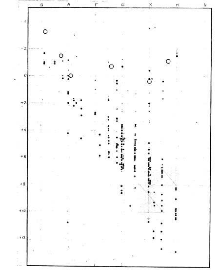
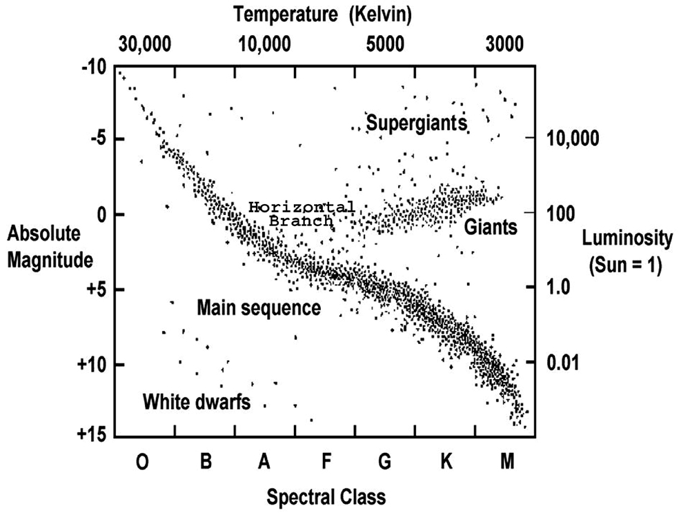
Hertzprung-Russell Diagram
Henry Russell's first diagram.
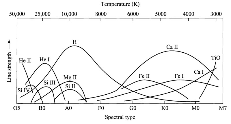
Spectral line strengths vs. temperature
Patterns were emerging in the spectral class system. The stars at the O end were both brighter and hotter than the M stars. Also, O stars were found to be more massive. The first idea, was that the spectral classes, O through M, represented the lifetime of the stars - that all stars started off big and hot, then cooled and got smaller over the years. This turned out to be incorrect.
Color & Temperature
The bolometric magnitudes discussed earlier were measures of the star's light emissions at all wavelengths. However, in practice, real measurements will take place in a range of wavelengths due to the sensitivities of the actual detectors.
We can measure the light from a star in 3 different wavelength windows:
$U$: the star's magnitude in the ultraviolet. ($f_c = 365 \; \textrm{nm}$, $f_{bw} = 68 \; \textrm{nm}$)
$B$: the star's magnitude in the blue region. ($f_c = 440 \; \textrm{nm}$, $f_{bw} = 98 \; \textrm{nm}$)
$V$: the star's magnitude in the visible region. ($f_c = 550 \; \textrm{nm}$, $f_{bw} = 89 \; \textrm{nm}$)
Color Index
$$\begin{equation}
T \approx \frac{9000 \; \textrm{K}}{(B-V)+0.93}
\end{equation}$$
Looking at the ratio of the B and V values, we can establish a temperature for the observed spectra.
HR Diagram
A Hertzsprung-Russell (H-R) Diagram showing the relationship between several star characteristics.
Maxwell-Boltzmann Velocity
$$\begin{equation}
n_v dv = n \left(\frac{m}{2 \pi kT}\right)^{3/2} \, 4\pi v^2 e^{- \frac{mv^2}{2kT}} dv
\label{eq:maxwell-boltzmann-distribution}
\end{equation}$$
The number of gas particles per unity volume having speeds between $v$ and $v+ dv$ is given by the Maxwell-Boltzmann velocity distribution . $n$ is the number of particles per unity volume (i.e. number density), $m$ is the particle's mass,
We can look at the exponent in the distribution to see where the peak of this function will occur. The exponent term is: $e^{- \frac{mv^2}{2kT}}$ which contains the kinetic energy: $\frac{1}{2}mv^2$ as well as the thermal energy: $kT$. The most probable speed will be when the kinetic energy is equal to the thermal energy. $\frac{1}{2}mv^2 = kT$:
$$\begin{equation}
v_{mp} = \sqrt{\frac{2kT}{m}}
\end{equation}$$
The rms value of the distribution: (square root of the average of $v^2$: $\sqrt{\bar{v^2}}$)
$$\begin{equation}
v_{\textrm{rms}} = \sqrt{ \frac{3 k T} {m}}
\end{equation}$$
Consider a gas of hydrogen atoms at 10000 K. What percentage of the atoms have speeds between 20000 m/s and 25000 m/s?
We have to integrate the MB function between these two limits. We could do this using a numerical integration.
  import numpy as np
  import scipy.integrate as integrate
  import scipy.constants as const
  mH = 1.6735e-27
  T = 10000
  f = lambda v : (mH/(2*np.pi*const.k*T))**(3/2)*np.exp(((-mH*v*v))/(2*const.k*T))*4*np.pi*v*v
  integrate.quad(f, 20000, 25000)
This yields an output of 0.12759 or about 12.8 % of the hydrogen atoms.